20. Xarray Fundamentals#
Attribution: This notebook is a revision of the Xarray Fundamentals notebook by Ryan Abernathy from An Introduction to Earth and Environmental Data Science.
In this lecture, we will have a deep dive to xarray package. So far in this class, we have used rioxarray for raster data processing, and stackstac for analyzing stacks of satellite imagery. Both of these packages are built on top of xarray; however, we didn’t use all the functionalities of xarray with them.
We also worked with xarray DataArray and Dataset after reading data from different sources. Here, we will learn how to create a DataArray or Dataset from scratch.
In the previous lecture on Raster Data Processing, we introduced Dataset in rioxarray and discussed how it is different from DataArray. Here we will have a complete review of data structures in xarray:
20.1. Xarray data structures#
Like Pandas, xarray has two fundamental data structures:
a
DataArray, which holds a single multi-dimensional variable and its coordinatesa
Dataset, which holds multiple variables that potentially share the same coordinates
20.1.1. DataArray#
A DataArray has four essential attributes:
values: anumpy.ndarrayholding the array’s valuesdims: dimension names for each axis (e.g.,('x', 'y', 'z'))coords: a dict-like container of arrays (coordinates) that label each point (e.g., 1-dimensional arrays of numbers, datetime objects or strings)attrs: anOrderedDictto hold arbitrary metadata (attributes)
Let’s start by constructing some DataArrays manually
import numpy as np
import xarray as xr
from matplotlib import pyplot as plt
A simple DataArray without dimensions or coordinates isn’t much use.
da = xr.DataArray([9, 0, 2, 1, 0])
da
<xarray.DataArray (dim_0: 5)>
array([9, 0, 2, 1, 0])
Dimensions without coordinates: dim_0
We can add a dimension name…
da = xr.DataArray([9, 0, 2, 1, 0], dims=['x'])
da
<xarray.DataArray (x: 5)>
array([9, 0, 2, 1, 0])
Dimensions without coordinates: x
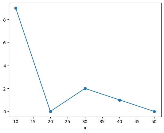
But things get most interesting when we add a coordinate:
da = xr.DataArray([9, 0, 2, 1, 0],
                  dims=['x'],
                  coords={'x': [10, 20, 30, 40, 50]})
da
<xarray.DataArray (x: 5)>
array([9, 0, 2, 1, 0])
Coordinates:
  * x        (x) int64 10 20 30 40 50
This coordinate has been used to create an index, which works very similar to a Pandas index. In fact, under the hood, Xarray just reuses Pandas indexes.
da.indexes
Indexes:
    x        Index([10, 20, 30, 40, 50], dtype='int64', name='x')
Xarray has built-in plotting, like pandas.
da.plot(marker='o')
[<matplotlib.lines.Line2D at 0x707006ab39d0>]
20.1.2. Multidimensional DataArray#
If we are just dealing with 1D data, Pandas and Xarray have very similar capabilities. Xarray’s real potential comes with multidimensional data.
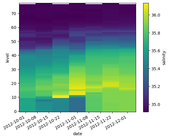
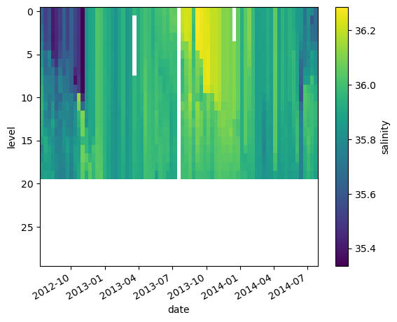
In this example, we use real data from ocean profiling floats. ARGO floats are autonomous robotic instruments that collect Temperature, Salinity, and Pressure data from the ocean. ARGO floats collect one “profile” (a set of messurements at different depths or “levels”).
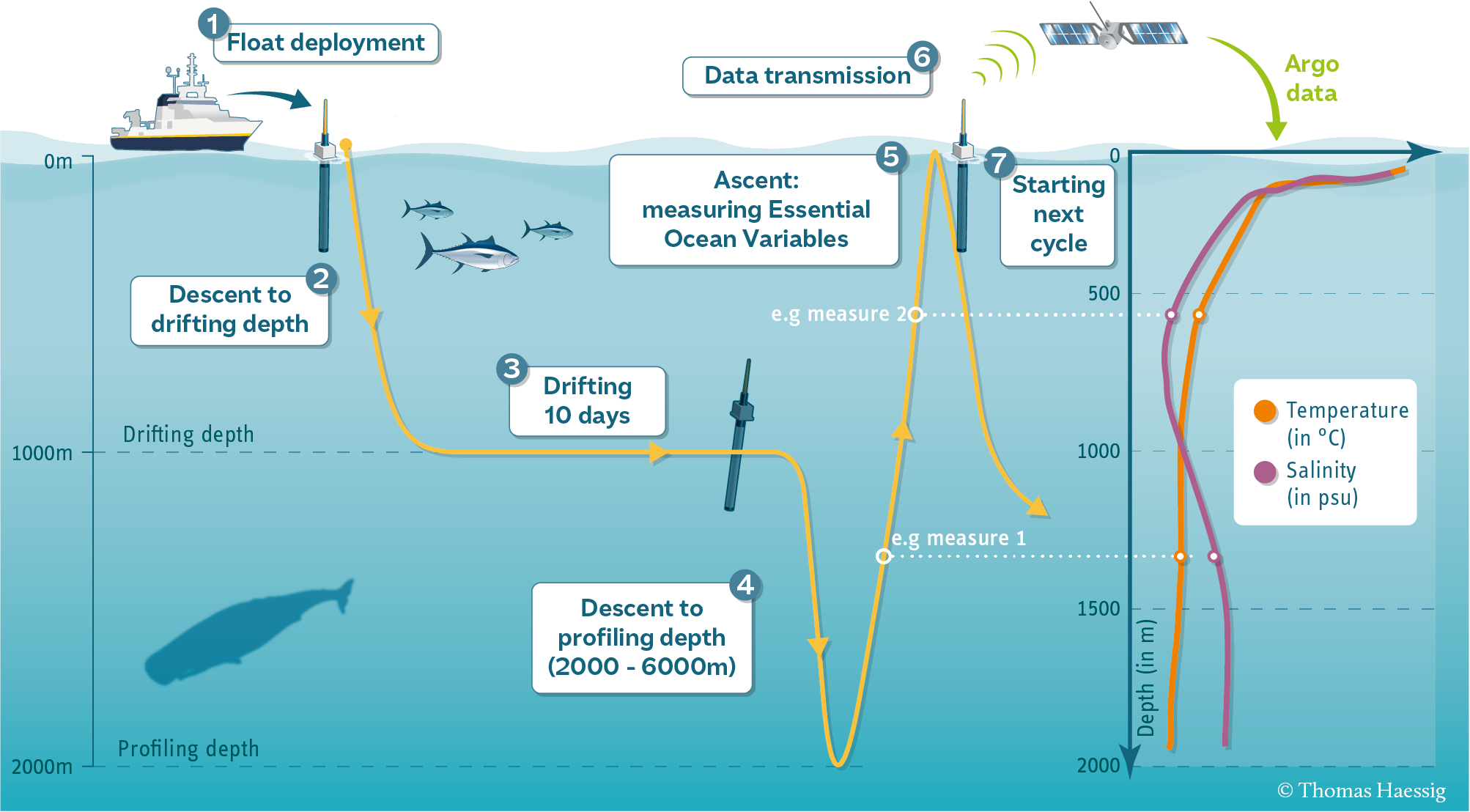
Each profile has a single latitude, longitude, and date associated with it, in addition to many different levels.
Let’s start by using pooch to download the data files we need for this exercise. The following code will give you a list of .npy files that you can open in the next step.
Note
You see that we are passing a hash to the retrieve method from pooch here. Hash-based verification ensures that a file has not been corrupted by comparing the file’s hash value to a previously calculated value. If these values match, the file is presumed to be unmodified.
import pooch
url = "https://www.ldeo.columbia.edu/~rpa/float_data_4901412.zip"
files = pooch.retrieve(url, processor=pooch.Unzip(), known_hash="2a703c720302c682f1662181d329c9f22f9f10e1539dc2d6082160a469165009")
files.sort()
files
['/home/jovyan/.cache/pooch/7e6685dbe2a3c0b0870f770f3ef413d9-float_data_4901412.zip.unzip/float_data/P.npy',
 '/home/jovyan/.cache/pooch/7e6685dbe2a3c0b0870f770f3ef413d9-float_data_4901412.zip.unzip/float_data/S.npy',
 '/home/jovyan/.cache/pooch/7e6685dbe2a3c0b0870f770f3ef413d9-float_data_4901412.zip.unzip/float_data/T.npy',
 '/home/jovyan/.cache/pooch/7e6685dbe2a3c0b0870f770f3ef413d9-float_data_4901412.zip.unzip/float_data/date.npy',
 '/home/jovyan/.cache/pooch/7e6685dbe2a3c0b0870f770f3ef413d9-float_data_4901412.zip.unzip/float_data/lat.npy',
 '/home/jovyan/.cache/pooch/7e6685dbe2a3c0b0870f770f3ef413d9-float_data_4901412.zip.unzip/float_data/levels.npy',
 '/home/jovyan/.cache/pooch/7e6685dbe2a3c0b0870f770f3ef413d9-float_data_4901412.zip.unzip/float_data/lon.npy']
We will manually load each of these variables into a numpy array. If this seems repetitive and inefficient, that’s the point! NumPy itself is not meant for managing groups of inter-related arrays. That’s what Xarray is for!
P = np.load(files[0])
S = np.load(files[1])
T = np.load(files[2])
date = np.load(files[3])
lat = np.load(files[4])
levels = np.load(files[5])
lon = np.load(files[6])
Let’s look at the shape of some of the variables:
print("Salinity shape is:", S.shape)
print("Levels shape is:", levels.shape)
print("Date shape is:", date.shape)
Salinity shape is: (78, 75)
Levels shape is: (78,)
Date shape is: (75,)
As expected, Salinity has dimensions of levels x date
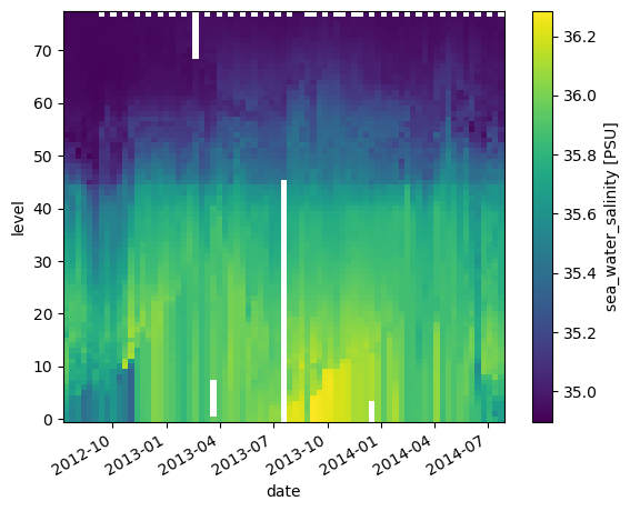
Let’s organize the data and coordinates of the salinity variable into a DataArray.
da_salinity = xr.DataArray(S, dims=['level', 'date'],
                           coords={'level': levels,
                                   'date': date},)
da_salinity
<xarray.DataArray (level: 78, date: 75)>
array([[35.6389389 , 35.51495743, 35.57297134, ..., 35.82093811,
        35.77793884, 35.66891098],
       [35.63393784, 35.5219574 , 35.57397079, ..., 35.81093216,
        35.58389664, 35.66791153],
       [35.6819458 , 35.52595901, 35.57297134, ..., 35.79592896,
        35.66290665, 35.66591263],
       ...,
       [34.91585922, 34.92390442, 34.92390442, ..., 34.93481064,
        34.94081116, 34.94680786],
       [34.91585922, 34.92390442, 34.92190552, ..., 34.93280792,
        34.93680954, 34.94380951],
       [34.91785812, 34.92390442, 34.92390442, ...,         nan,
        34.93680954,         nan]])
Coordinates:
  * level    (level) int64 0 1 2 3 4 5 6 7 8 9 ... 68 69 70 71 72 73 74 75 76 77
* date (date) datetime64[ns] 2012-07-13T22:33:06.019200 ... 2014-07-24T...da_salinity.plot()
<matplotlib.collections.QuadMesh at 0x706ffe11b110>
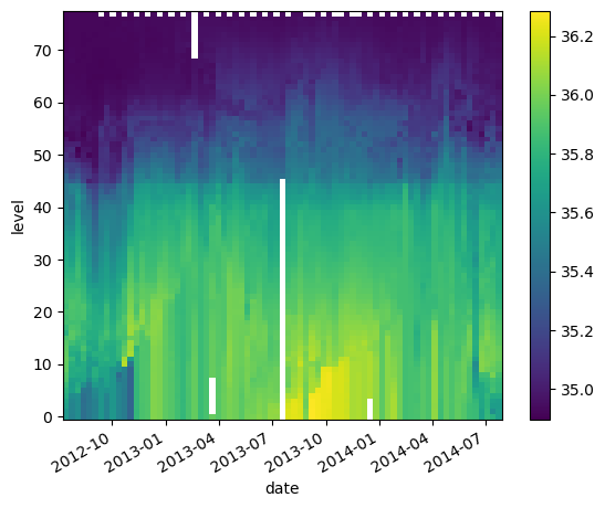
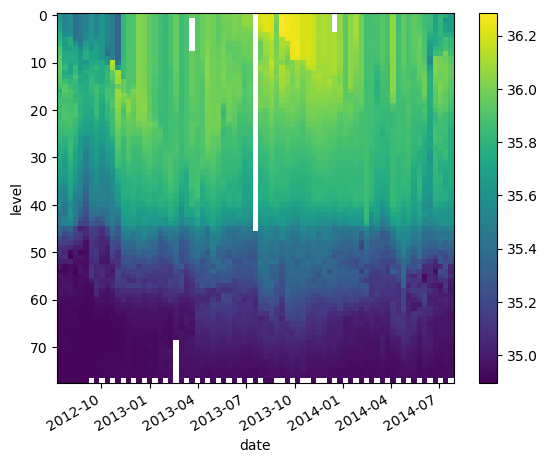
Since we are working with ocean data, it’s helpful to plot the level in an increasing order from top to bottom:
da_salinity.plot(yincrease=False)
<matplotlib.collections.QuadMesh at 0x706ffdfd7cd0>
Attributes can be used to store metadata. What metadata should you store? The CF Conventions are a great resource for thinking about climate metadata. Below we define two of the required CF-conventions attributes.
da_salinity.attrs['units'] = 'PSU'
da_salinity.attrs['standard_name'] = 'sea_water_salinity'
da_salinity
<xarray.DataArray (level: 78, date: 75)>
array([[35.6389389 , 35.51495743, 35.57297134, ..., 35.82093811,
        35.77793884, 35.66891098],
       [35.63393784, 35.5219574 , 35.57397079, ..., 35.81093216,
        35.58389664, 35.66791153],
       [35.6819458 , 35.52595901, 35.57297134, ..., 35.79592896,
        35.66290665, 35.66591263],
       ...,
       [34.91585922, 34.92390442, 34.92390442, ..., 34.93481064,
        34.94081116, 34.94680786],
       [34.91585922, 34.92390442, 34.92190552, ..., 34.93280792,
        34.93680954, 34.94380951],
       [34.91785812, 34.92390442, 34.92390442, ...,         nan,
        34.93680954,         nan]])
Coordinates:
* level (level) int64 0 1 2 3 4 5 6 7 8 9 ... 68 69 70 71 72 73 74 75 76 77
* date (date) datetime64[ns] 2012-07-13T22:33:06.019200 ... 2014-07-24T...
Attributes:
units: PSU
standard_name: sea_water_salinityNow if we plot the data again, the name and units are automatically attached to the figure.
da_salinity.plot()
<matplotlib.collections.QuadMesh at 0x706ffde8fcd0>
20.1.3. Datasets#
A Dataset holds many DataArrays which potentially can share coordinates. In analogy to pandas:
pandas.Series : pandas.Dataframe :: xarray.DataArray : xarray.Dataset
Constructing Datasets manually is a bit more involved in terms of syntax. The Dataset constructor takes three arguments:
data_varsshould be a dictionary with each key as the name of the variable and each value as one of:A
DataArrayor VariableA tuple of the form
(dims, data[, attrs]), which is converted into arguments for VariableA pandas object, which is converted into a
DataArrayA 1D array or list, which is interpreted as values for a one dimensional coordinate variable along the same dimension as it’s name
coordsshould be a dictionary of the same form as data_vars.attrsshould be a dictionary.
Let’s put together a Dataset with temperature, salinity and pressure all together
argo = xr.Dataset(
data_vars={
'salinity': (('level', 'date'), S),
'temperature': (('level', 'date'), T),
'pressure': (('level', 'date'), P)
},
coords={
'level': levels,
'date': date
}
)
argo
<xarray.Dataset>
Dimensions: (level: 78, date: 75)
Coordinates:
* level (level) int64 0 1 2 3 4 5 6 7 8 ... 69 70 71 72 73 74 75 76 77
* date (date) datetime64[ns] 2012-07-13T22:33:06.019200 ... 2014-07...
Data variables:
salinity (level, date) float64 35.64 35.51 35.57 35.4 ... nan 34.94 nan
temperature (level, date) float64 18.97 18.44 19.1 19.79 ... nan 3.714 nan
pressure (level, date) float64 6.8 6.1 6.5 5.0 ... 2e+03 nan 2e+03 nanWhat about lon and lat? We forgot them in the creation process, but we can add them after the fact.
argo.coords['lon'] = lon
argo
<xarray.Dataset>
Dimensions: (level: 78, date: 75, lon: 75)
Coordinates:
* level (level) int64 0 1 2 3 4 5 6 7 8 ... 69 70 71 72 73 74 75 76 77
* date (date) datetime64[ns] 2012-07-13T22:33:06.019200 ... 2014-07...
* lon (lon) float64 -39.13 -37.28 -36.9 ... -33.83 -34.11 -34.38
Data variables:
salinity (level, date) float64 35.64 35.51 35.57 35.4 ... nan 34.94 nan
temperature (level, date) float64 18.97 18.44 19.1 19.79 ... nan 3.714 nan
pressure (level, date) float64 6.8 6.1 6.5 5.0 ... 2e+03 nan 2e+03 nanThat was not quite right…we want lon to have dimension date:
del argo['lon']
argo.coords['lon'] = ('date', lon)
argo.coords['lat'] = ('date', lat)
argo
<xarray.Dataset>
Dimensions: (level: 78, date: 75)
Coordinates:
* level (level) int64 0 1 2 3 4 5 6 7 8 ... 69 70 71 72 73 74 75 76 77
* date (date) datetime64[ns] 2012-07-13T22:33:06.019200 ... 2014-07...
lon (date) float64 -39.13 -37.28 -36.9 ... -33.83 -34.11 -34.38
lat (date) float64 47.19 46.72 46.45 46.23 ... 42.6 42.46 42.38
Data variables:
salinity (level, date) float64 35.64 35.51 35.57 35.4 ... nan 34.94 nan
temperature (level, date) float64 18.97 18.44 19.1 19.79 ... nan 3.714 nan
pressure (level, date) float64 6.8 6.1 6.5 5.0 ... 2e+03 nan 2e+03 nan20.1.4. Coordinates vs. Data Variables#
Data variables can be modified through arithmentic operations or other functions. Coordinates are always keept the same.
argo * 10000
<xarray.Dataset>
Dimensions: (level: 78, date: 75)
Coordinates:
* level (level) int64 0 1 2 3 4 5 6 7 8 ... 69 70 71 72 73 74 75 76 77
* date (date) datetime64[ns] 2012-07-13T22:33:06.019200 ... 2014-07...
lon (date) float64 -39.13 -37.28 -36.9 ... -33.83 -34.11 -34.38
lat (date) float64 47.19 46.72 46.45 46.23 ... 42.6 42.46 42.38
Data variables:
salinity (level, date) float64 3.564e+05 3.551e+05 ... 3.494e+05 nan
temperature (level, date) float64 1.897e+05 1.844e+05 ... 3.714e+04 nan
pressure (level, date) float64 6.8e+04 6.1e+04 6.5e+04 ... nan 2e+07 nanClearly lon and lat are coordinates rather than data variables.
The bold font in the representation above indicates that level and date are “dimension coordinates” (they describe the coordinates associated with data variable axes) while lon and lat are “non-dimension coordinates”. We can make any variable a non-dimension coordiante (using set_coords).
20.2. Selecting Data (Indexing)#
We can always use regular numpy indexing and slicing on DataArrays
argo.salinity.shape
(78, 75)
argo.salinity[2]
<xarray.DataArray 'salinity' (date: 75)>
array([35.6819458 , 35.52595901, 35.57297134, 35.40494537, 35.45091629,
35.50192261, 35.62397766, 35.51696014, 35.62797546, 35.52292252,
35.47383118, 35.33785629, 35.81896591, 35.88694 , 35.90187836,
36.02391815, 36.00475693, 35.94187927, 35.91583252, 35.86392212,
35.81995392, 35.88601303, 35.95079422, 35.84091568, 35.87992477,
nan, 35.92179108, 35.96979141, 36.0008316 , 35.98083115,
35.92887878, 35.98091888, 35.9838829 , 36.01884842, 35.99092484,
36.04689026, 36.04185867, nan, 36.19193268, 36.22789764,
36.20986557, 35.97589874, 36.2779007 , 36.25889969, 36.2418251 ,
36.23685837, 36.19781876, 36.19785309, 36.17692184, 36.1048851 ,
36.11392212, 36.09080505, nan, 36.05675888, 35.93374634,
36.04291534, 36.10183716, 35.97779083, 35.86592102, 35.87791824,
35.88392258, 35.92078781, 35.88601303, 36.05178833, 35.85883713,
35.94878769, 35.8938446 , 35.94379425, 35.90884018, 35.84893036,
35.83496857, 35.71691132, 35.79592896, 35.66290665, 35.66591263])
Coordinates:
level int64 2
* date (date) datetime64[ns] 2012-07-13T22:33:06.019200 ... 2014-07-24T...
lon (date) float64 -39.13 -37.28 -36.9 -36.89 ... -33.83 -34.11 -34.38
lat (date) float64 47.19 46.72 46.45 46.23 ... 42.72 42.6 42.46 42.38argo.salinity[2].plot()
[<matplotlib.lines.Line2D at 0x706ffdda6a10>]
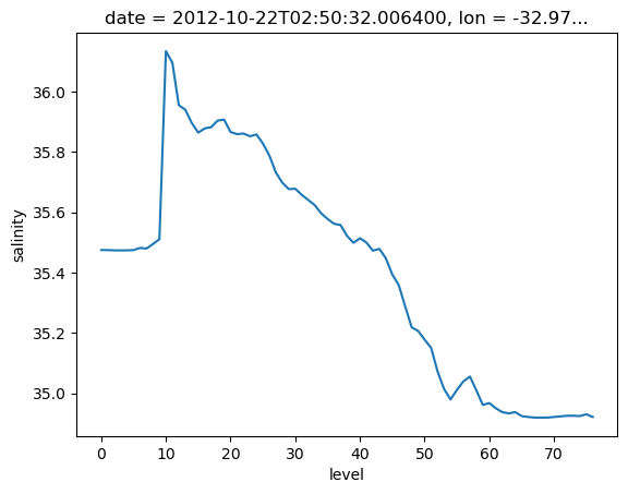
argo.salinity[:, 10]
<xarray.DataArray 'salinity' (level: 78)>
array([35.47483063, 35.47483063, 35.47383118, 35.47383118, 35.47383118,
35.47483063, 35.48183441, 35.47983551, 35.4948349 , 35.51083755,
36.13380051, 36.09579849, 35.95479965, 35.93979645, 35.8958931 ,
35.86388397, 35.87788773, 35.88188934, 35.90379333, 35.9067955 ,
35.86588669, 35.8588829 , 35.86088181, 35.85188293, 35.85788345,
35.82787323, 35.78786469, 35.73185349, 35.69784927, 35.67684174,
35.677845 , 35.65784073, 35.64083481, 35.6238327 , 35.59682846,
35.57782364, 35.56182098, 35.55781937, 35.52181625, 35.49881363,
35.51381302, 35.49981308, 35.47280884, 35.47880936, 35.44780731,
35.39379501, 35.35879135, 35.28778076, 35.21878052, 35.20677567,
35.17777252, 35.15076828, 35.07276535, 35.01475525, 34.9797554 ,
35.0117569 , 35.03975677, 35.05575562, 35.00975037, 34.96175385,
34.96775055, 34.95075226, 34.93775177, 34.93375015, 34.93775558,
34.9247551 , 34.92175674, 34.91975403, 34.91975403, 34.91975403,
34.92176056, 34.92375946, 34.92575836, 34.92575836, 34.92475891,
34.93076324, 34.92176437, nan])
Coordinates:
* level (level) int64 0 1 2 3 4 5 6 7 8 9 ... 68 69 70 71 72 73 74 75 76 77
date datetime64[ns] 2012-10-22T02:50:32.006400
lon float64 -32.97
lat float64 44.13argo.salinity[:, 10:11].plot()
[<matplotlib.lines.Line2D at 0x706ffd617690>]
However, it is often much more powerful to use xarray’s .sel() method to use label-based indexing.
argo.salinity.sel(level=[2, 5])
<xarray.DataArray 'salinity' (level: 2, date: 75)>
array([[35.6819458 , 35.52595901, 35.57297134, 35.40494537, 35.45091629,
35.50192261, 35.62397766, 35.51696014, 35.62797546, 35.52292252,
35.47383118, 35.33785629, 35.81896591, 35.88694 , 35.90187836,
36.02391815, 36.00475693, 35.94187927, 35.91583252, 35.86392212,
35.81995392, 35.88601303, 35.95079422, 35.84091568, 35.87992477,
nan, 35.92179108, 35.96979141, 36.0008316 , 35.98083115,
35.92887878, 35.98091888, 35.9838829 , 36.01884842, 35.99092484,
36.04689026, 36.04185867, nan, 36.19193268, 36.22789764,
36.20986557, 35.97589874, 36.2779007 , 36.25889969, 36.2418251 ,
36.23685837, 36.19781876, 36.19785309, 36.17692184, 36.1048851 ,
36.11392212, 36.09080505, nan, 36.05675888, 35.93374634,
36.04291534, 36.10183716, 35.97779083, 35.86592102, 35.87791824,
35.88392258, 35.92078781, 35.88601303, 36.05178833, 35.85883713,
35.94878769, 35.8938446 , 35.94379425, 35.90884018, 35.84893036,
35.83496857, 35.71691132, 35.79592896, 35.66290665, 35.66591263],
[35.7889595 , 35.67097855, 35.77500153, 35.4429512 , 35.44491196,
35.55392838, 35.62497711, 35.59697342, 35.62897873, 35.52292252,
35.47483063, 35.33785629, 35.81996536, 35.88993835, 35.90187836,
36.02191925, 36.00475693, 35.93987656, 35.91583633, 35.86492538,
35.81995773, 35.8870163 , 35.95079422, 35.84191513, 35.87992477,
nan, 35.92179108, 35.96479034, 36.00683594, 35.98083115,
35.9368782 , 35.99091721, 35.962883 , 35.98684311, 35.97792435,
35.98988724, 35.97084808, nan, 36.0339241 , 36.09988785,
36.15286255, 35.98789215, 36.11489487, 36.24489975, 36.24282455,
36.24985886, 36.19781876, 36.19885254, 36.17592239, 36.10388565,
36.11192322, 36.09080505, 36.11088181, 36.05976105, 35.93475342,
36.04491425, 36.08283615, 35.97679138, 35.86592102, 35.87791824,
35.88392258, 35.92078781, 35.88500977, 36.0527916 , 35.87383652,
35.9487915 , 35.8938446 , 35.9407959 , 35.97483444, 35.87393188,
35.73094177, 35.73391342, 35.77991486, 35.87294388, 35.8139267 ]])
Coordinates:
* level (level) int64 2 5
* date (date) datetime64[ns] 2012-07-13T22:33:06.019200 ... 2014-07-24T...
lon (date) float64 -39.13 -37.28 -36.9 -36.89 ... -33.83 -34.11 -34.38
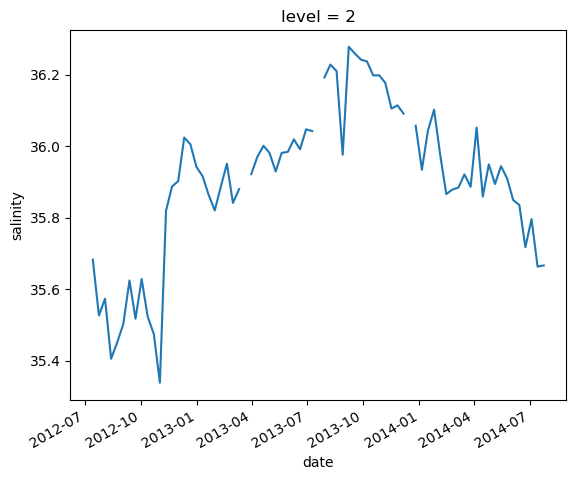
lat (date) float64 47.19 46.72 46.45 46.23 ... 42.72 42.6 42.46 42.38argo.salinity.sel(level=2)
<xarray.DataArray 'salinity' (date: 75)>
array([35.6819458 , 35.52595901, 35.57297134, 35.40494537, 35.45091629,
35.50192261, 35.62397766, 35.51696014, 35.62797546, 35.52292252,
35.47383118, 35.33785629, 35.81896591, 35.88694 , 35.90187836,
36.02391815, 36.00475693, 35.94187927, 35.91583252, 35.86392212,
35.81995392, 35.88601303, 35.95079422, 35.84091568, 35.87992477,
nan, 35.92179108, 35.96979141, 36.0008316 , 35.98083115,
35.92887878, 35.98091888, 35.9838829 , 36.01884842, 35.99092484,
36.04689026, 36.04185867, nan, 36.19193268, 36.22789764,
36.20986557, 35.97589874, 36.2779007 , 36.25889969, 36.2418251 ,
36.23685837, 36.19781876, 36.19785309, 36.17692184, 36.1048851 ,
36.11392212, 36.09080505, nan, 36.05675888, 35.93374634,
36.04291534, 36.10183716, 35.97779083, 35.86592102, 35.87791824,
35.88392258, 35.92078781, 35.88601303, 36.05178833, 35.85883713,
35.94878769, 35.8938446 , 35.94379425, 35.90884018, 35.84893036,
35.83496857, 35.71691132, 35.79592896, 35.66290665, 35.66591263])
Coordinates:
level int64 2
* date (date) datetime64[ns] 2012-07-13T22:33:06.019200 ... 2014-07-24T...
lon (date) float64 -39.13 -37.28 -36.9 -36.89 ... -33.83 -34.11 -34.38
lat (date) float64 47.19 46.72 46.45 46.23 ... 42.72 42.6 42.46 42.38Under the hood, this method is powered by using pandas’s powerful Index objects which means this method uses pandas’s (well documented) logic for indexing. For example, you can use string shortcuts for datetime indexes (e.g., ‘2000-01’ to select all values in January 2000). It also means that slices are treated as inclusive of both the start and stop values, unlike normal Python indexing.
argo.salinity.sel(level=2).plot()
[<matplotlib.lines.Line2D at 0x706ffdcbb5d0>]
argo.salinity.sel(date='2012-10-22')
<xarray.DataArray 'salinity' (level: 78, date: 1)>
array([[35.47483063],
[35.47483063],
[35.47383118],
[35.47383118],
[35.47383118],
[35.47483063],
[35.48183441],
[35.47983551],
[35.4948349 ],
[35.51083755],
[36.13380051],
[36.09579849],
[35.95479965],
[35.93979645],
[35.8958931 ],
[35.86388397],
[35.87788773],
[35.88188934],
[35.90379333],
[35.9067955 ],
...
[35.00975037],
[34.96175385],
[34.96775055],
[34.95075226],
[34.93775177],
[34.93375015],
[34.93775558],
[34.9247551 ],
[34.92175674],
[34.91975403],
[34.91975403],
[34.91975403],
[34.92176056],
[34.92375946],
[34.92575836],
[34.92575836],
[34.92475891],
[34.93076324],
[34.92176437],
[ nan]])
Coordinates:
* level (level) int64 0 1 2 3 4 5 6 7 8 9 ... 68 69 70 71 72 73 74 75 76 77
* date (date) datetime64[ns] 2012-10-22T02:50:32.006400
lon (date) float64 -32.97
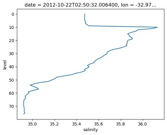
lat (date) float64 44.13We can improve the plot by using the yincrease argument, and setting the variable that will be plotted on y axis:
argo.salinity.sel(date='2012-10-22').plot(y='level', yincrease=False)
[<matplotlib.lines.Line2D at 0x706ffdce3d90>]
.sel() also supports slicing. Unfortunately we have to use a somewhat awkward syntax, but it still works.
argo.salinity.sel(date=slice('2012-10-01', '2012-12-01'))
<xarray.DataArray 'salinity' (level: 78, date: 7)>
array([[35.63097763, 35.52592468, 35.47483063, 35.33785629, 35.81896591,
35.8889389 , 35.90187836],
[35.63097763, 35.52292252, 35.47483063, 35.33685684, 35.81796646,
35.88793945, 35.90187836],
[35.62797546, 35.52292252, 35.47383118, 35.33785629, 35.81896591,
35.88694 , 35.90187836],
[35.62697601, 35.52192307, 35.47383118, 35.33785629, 35.81896591,
35.89193726, 35.90187836],
[35.62797546, 35.52192307, 35.47383118, 35.33785629, 35.81996536,
35.88993835, 35.90187836],
[35.62897873, 35.52292252, 35.47483063, 35.33785629, 35.81996536,
35.88993835, 35.90187836],
[35.62997818, 35.51892471, 35.48183441, 35.33785629, 35.81996536,
35.88993835, 35.90187836],
[35.63197708, 35.44991302, 35.47983551, 35.33785629, 35.81996536,
35.89683914, 35.90187836],
[35.63097763, 35.38090134, 35.4948349 , 35.33785629, 35.81896591,
35.89583969, 35.90187836],
[35.62697601, 35.58792114, 35.51083755, 35.33985519, 35.82497025,
35.89683914, 35.90187836],
...
[34.91690445, 34.92385483, 34.91975403, 34.91980362, 34.92385483,
34.93680573, 34.93885422],
[34.92190552, 34.92485428, 34.91975403, 34.92080688, 34.92485428,
34.94480515, 34.9328537 ],
[34.92390442, 34.92285538, 34.92176056, 34.92280579, 34.92985535,
34.93280411, 34.92785645],
[34.92390442, 34.92385483, 34.92375946, 34.92480469, 34.92685318,
34.93780899, 34.92485428],
[34.92390442, 34.92285538, 34.92575836, 34.92181015, 34.92085648,
34.93680954, 34.92385483],
[34.92590332, 34.9288559 , 34.92575836, 34.92181015, 34.92685318,
34.93481064, 34.92585373],
[34.92490387, 34.92785645, 34.92475891, 34.92781067, 34.93385696,
34.93380737, 34.92385864],
[34.92190552, 34.92385864, 34.93076324, 34.9268074 , 34.93585968,
34.93481064, 34.92985916],
[34.92090607, 34.92185974, 34.92176437, 34.9228096 , 34.93285751,
34.93180847, 34.92786026],
[ nan, 34.91985703, nan, 34.92181015, nan,
34.92181015, nan]])
Coordinates:
* level (level) int64 0 1 2 3 4 5 6 7 8 9 ... 68 69 70 71 72 73 74 75 76 77
* date (date) datetime64[ns] 2012-10-02T03:00:17.971200 ... 2012-12-01T...
lon (date) float64 -34.46 -33.78 -32.97 -32.55 -32.43 -32.29 -32.17
lat (date) float64 44.96 44.68 44.13 43.64 43.07 42.66 42.51argo.salinity.sel(date=slice('2012-10-01', '2012-12-01')).plot()
<matplotlib.collections.QuadMesh at 0x706ffdcaee90>
.sel() also works on the whole Dataset
argo.sel(date='2012-10-22')
<xarray.Dataset>
Dimensions: (level: 78, date: 1)
Coordinates:
* level (level) int64 0 1 2 3 4 5 6 7 8 ... 69 70 71 72 73 74 75 76 77
* date (date) datetime64[ns] 2012-10-22T02:50:32.006400
lon (date) float64 -32.97
lat (date) float64 44.13
Data variables:
salinity (level, date) float64 35.47 35.47 35.47 ... 34.93 34.92 nan
temperature (level, date) float64 17.13 17.13 17.13 ... 3.736 3.639 nan
pressure (level, date) float64 6.4 10.3 15.4 ... 1.9e+03 1.951e+03 nanargo.sel(date = '2012-12-22')
<xarray.Dataset>
Dimensions: (level: 78, date: 0)
Coordinates:
* level (level) int64 0 1 2 3 4 5 6 7 8 ... 69 70 71 72 73 74 75 76 77
* date (date) datetime64[ns]
lon (date) float64
lat (date) float64
Data variables:
salinity (level, date) float64
temperature (level, date) float64
pressure (level, date) float64 20.3. Computation#
Xarray DataArrays and Datasets work seamlessly with arithmetic operators and numpy array functions.
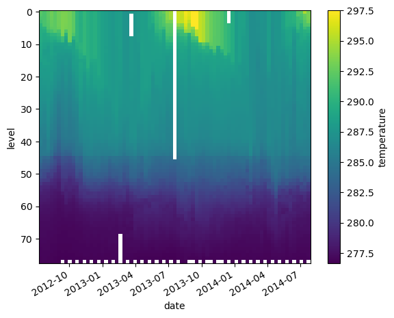
temp_kelvin = argo.temperature + 273.15
temp_kelvin.plot(yincrease=False)
<matplotlib.collections.QuadMesh at 0x706ffdc6eed0>
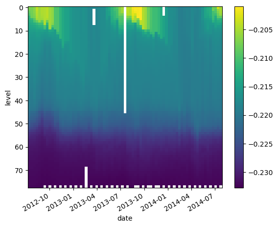
We can also combine multiple xarray datasets in arithemtic operations
g = 9.8
buoyancy = g * (2e-4 * argo.temperature - 7e-4 * argo.salinity)
buoyancy.plot(yincrease=False)
<matplotlib.collections.QuadMesh at 0x706ffdec04d0>
20.4. Broadcasting, Aligment, and Combining Data#
20.4.1. Broadcasting#
Broadcasting arrays in numpy is a nightmare. It is much easier when the data axes are labeled!
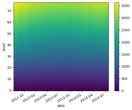
This is a useless calculation, but it illustrates how perfoming an operation on arrays with differenty coordinates will result in automatic broadcasting
argo.level
<xarray.DataArray 'level' (level: 78)>
array([ 0,  1,  2,  3,  4,  5,  6,  7,  8,  9, 10, 11, 12, 13, 14, 15, 16, 17,
       18, 19, 20, 21, 22, 23, 24, 25, 26, 27, 28, 29, 30, 31, 32, 33, 34, 35,
       36, 37, 38, 39, 40, 41, 42, 43, 44, 45, 46, 47, 48, 49, 50, 51, 52, 53,
       54, 55, 56, 57, 58, 59, 60, 61, 62, 63, 64, 65, 66, 67, 68, 69, 70, 71,
       72, 73, 74, 75, 76, 77])
Coordinates:
* level (level) int64 0 1 2 3 4 5 6 7 8 9 ... 68 69 70 71 72 73 74 75 76 77argo.lat
<xarray.DataArray 'lat' (date: 75)>
array([47.187, 46.716, 46.45 , 46.23 , 45.459, 44.833, 44.452, 44.839,
       44.956, 44.676, 44.13 , 43.644, 43.067, 42.662, 42.513, 42.454,
       42.396, 42.256, 42.089, 41.944, 41.712, 41.571, 41.596, 41.581,
       41.351, 41.032, 40.912, 40.792, 40.495, 40.383, 40.478, 40.672,
       41.032, 40.864, 40.651, 40.425, 40.228, 40.197, 40.483, 40.311,
       40.457, 40.463, 40.164, 40.047, 39.963, 40.122, 40.57 , 40.476,
       40.527, 40.589, 40.749, 40.993, 41.162, 41.237, 41.448, 41.65 ,
       42.053, 42.311, 42.096, 41.683, 41.661, 41.676, 42.018, 42.395,
       42.532, 42.558, 42.504, 42.63 , 42.934, 42.952, 42.777, 42.722,
       42.601, 42.457, 42.379])
Coordinates:
* date (date) datetime64[ns] 2012-07-13T22:33:06.019200 ... 2014-07-24T...
lon (date) float64 -39.13 -37.28 -36.9 -36.89 ... -33.83 -34.11 -34.38
lat (date) float64 47.19 46.72 46.45 46.23 ... 42.72 42.6 42.46 42.38level_times_lat = argo.level * argo.lat
level_times_lat
<xarray.DataArray (level: 78, date: 75)>
array([[   0.   ,    0.   ,    0.   , ...,    0.   ,    0.   ,    0.   ],
       [  47.187,   46.716,   46.45 , ...,   42.601,   42.457,   42.379],
       [  94.374,   93.432,   92.9  , ...,   85.202,   84.914,   84.758],
       ...,
       [3539.025, 3503.7  , 3483.75 , ..., 3195.075, 3184.275, 3178.425],
       [3586.212, 3550.416, 3530.2  , ..., 3237.676, 3226.732, 3220.804],
       [3633.399, 3597.132, 3576.65 , ..., 3280.277, 3269.189, 3263.183]])
Coordinates:
  * level    (level) int64 0 1 2 3 4 5 6 7 8 9 ... 68 69 70 71 72 73 74 75 76 77
  * date     (date) datetime64[ns] 2012-07-13T22:33:06.019200 ... 2014-07-24T...
    lon      (date) float64 -39.13 -37.28 -36.9 -36.89 ... -33.83 -34.11 -34.38
lat (date) float64 47.19 46.72 46.45 46.23 ... 42.72 42.6 42.46 42.38level_times_lat.plot()
<matplotlib.collections.QuadMesh at 0x706ffda92150>
20.4.2. Alignment#
If you try to perform operations on DataArrays that share a dimension name, Xarray will try to align them first.
This works nearly identically to Pandas, except that there can be multiple dimensions to align over.
To see how alignment works, we will create some subsets of our original data.
sa_surf = argo.salinity.isel(level=slice(0, 20))
sa_mid = argo.salinity.isel(level=slice(10, 30))
By default, when we combine multiple arrays in mathematical operations, Xarray performs an “inner join”.
(sa_surf * sa_mid).level
<xarray.DataArray 'level' (level: 10)>
array([10, 11, 12, 13, 14, 15, 16, 17, 18, 19])
Coordinates:
  * level    (level) int64 10 11 12 13 14 15 16 17 18 19
We can override this behavior by manually aligning the data
sa_surf_outer, sa_mid_outer = xr.align(sa_surf, sa_mid, join='outer')
sa_surf_outer
<xarray.DataArray 'salinity' (level: 30, date: 75)>
array([[35.6389389 , 35.51495743, 35.57297134, ..., 35.82093811,
        35.77793884, 35.66891098],
       [35.63393784, 35.5219574 , 35.57397079, ..., 35.81093216,
        35.58389664, 35.66791153],
       [35.6819458 , 35.52595901, 35.57297134, ..., 35.79592896,
        35.66290665, 35.66591263],
       ...,
       [        nan,         nan,         nan, ...,         nan,
                nan,         nan],
       [        nan,         nan,         nan, ...,         nan,
                nan,         nan],
       [        nan,         nan,         nan, ...,         nan,
                nan,         nan]])
Coordinates:
  * level    (level) int64 0 1 2 3 4 5 6 7 8 9 ... 20 21 22 23 24 25 26 27 28 29
  * date     (date) datetime64[ns] 2012-07-13T22:33:06.019200 ... 2014-07-24T...
    lon      (date) float64 -39.13 -37.28 -36.9 -36.89 ... -33.83 -34.11 -34.38
lat (date) float64 47.19 46.72 46.45 46.23 ... 42.72 42.6 42.46 42.38As we can see, missing data (NaNs) have been filled in where the array was extended.
From the documentation: Missing values (if join != 'inner') are filled with fill_value. The default fill value is NaN.
sa_surf_outer.plot(yincrease=False)
<matplotlib.collections.QuadMesh at 0x706ffd907010>
We can also use join='right' and join='left'.
If we run our multiplication on the aligned data:
(sa_surf_outer * sa_mid_outer).level
<xarray.DataArray 'level' (level: 30)>
array([ 0,  1,  2,  3,  4,  5,  6,  7,  8,  9, 10, 11, 12, 13, 14, 15, 16, 17,
       18, 19, 20, 21, 22, 23, 24, 25, 26, 27, 28, 29])
Coordinates:
* level (level) int64 0 1 2 3 4 5 6 7 8 9 ... 20 21 22 23 24 25 26 27 28 2920.4.3. Combing Data: Concat and Merge#
The ability to combine many smaller arrays into a single big Dataset is one of the main advantages of Xarray.
To take advantage of this, we need to learn two operations that help us combine data:
xr.contact: to concatenate multiple arrays into one bigger array along their dimensionsxr.merge: to combine multiple different arrays into a dataset
First let’s look at concat. Let’s re-combine the subsetted data from the previous step.
sa_surf_mid = xr.concat([sa_surf, sa_mid], dim='level')
sa_surf_mid
<xarray.DataArray 'salinity' (level: 40, date: 75)>
array([[35.6389389 , 35.51495743, 35.57297134, ..., 35.82093811,
        35.77793884, 35.66891098],
       [35.63393784, 35.5219574 , 35.57397079, ..., 35.81093216,
        35.58389664, 35.66791153],
       [35.6819458 , 35.52595901, 35.57297134, ..., 35.79592896,
        35.66290665, 35.66591263],
       ...,
       [35.78895187, 35.7829895 , 35.85100555, ..., 35.84291458,
        35.81891251, 35.7779007 ],
       [35.76794815, 35.75598526, 35.84500504, ..., 35.84891891,
        35.83391571, 35.76390076],
       [35.75194168, 35.71097565, 35.83100128, ..., 35.80690765,
        35.85292053, 35.75489807]])
Coordinates:
  * level    (level) int64 0 1 2 3 4 5 6 7 8 9 ... 20 21 22 23 24 25 26 27 28 29
  * date     (date) datetime64[ns] 2012-07-13T22:33:06.019200 ... 2014-07-24T...
    lon      (date) float64 -39.13 -37.28 -36.9 -36.89 ... -33.83 -34.11 -34.38
lat (date) float64 47.19 46.72 46.45 46.23 ... 42.72 42.6 42.46 42.38Warning
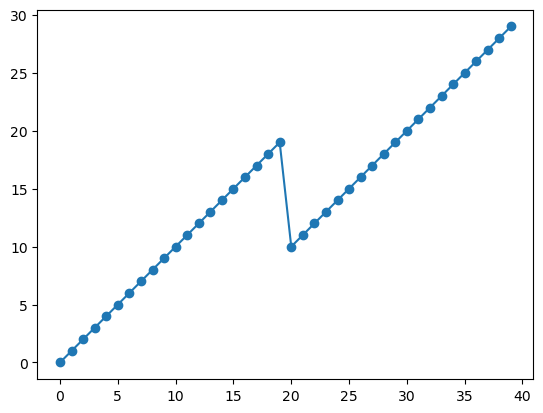
Xarray won’t check the values of the coordinates before concat. It will just stick everything together into a new array.
In this case, we had overlapping data. We can see this by looking at the level coordinate.
sa_surf_mid.level
<xarray.DataArray 'level' (level: 40)>
array([ 0,  1,  2,  3,  4,  5,  6,  7,  8,  9, 10, 11, 12, 13, 14, 15, 16, 17,
       18, 19, 10, 11, 12, 13, 14, 15, 16, 17, 18, 19, 20, 21, 22, 23, 24, 25,
       26, 27, 28, 29])
Coordinates:
* level (level) int64 0 1 2 3 4 5 6 7 8 9 ... 20 21 22 23 24 25 26 27 28 29sa_surf_mid.sel(level=11)
<xarray.DataArray 'salinity' (level: 2, date: 75)>
array([[35.95887756, 35.82500458, 35.70597839, 35.8350029 , 35.64592743,
        35.71894073, 35.76799011, 35.80199432, 35.7379837 , 35.79395294,
        36.09579849, 35.6628952 , 35.83797073, 35.89783859, 35.89887619,
        36.02391815, 36.00475693, 35.94387817, 35.90093613, 35.85692215,
        35.81895828, 35.86300659, 35.94979477, 35.84291458, 35.87992477,
        35.95978928, 35.92179108, 35.94578934, 36.04083633, 35.98183441,
        35.96687317, 35.99791718, 35.96387863, 35.9588356 , 35.95691681,
        35.91187668, 35.93383408,         nan, 36.06692123, 36.05187607,
        36.12983704, 36.01087952, 36.13287735, 36.02987671, 36.01980209,
        36.09484482, 36.02880096, 36.13484573, 36.15492249, 36.08387756,
        36.09292221, 36.09080505, 36.10988235, 36.05976105, 35.9327507 ,
        36.04291534, 36.01783371, 35.97879028, 35.86592102, 35.87792206,
        35.82791138, 35.89588547, 35.86800766, 36.05178833, 35.87783432,
        35.9337883 , 35.8938446 , 35.88488388, 35.95883179, 35.94283676,
        35.67092896, 36.02183533, 35.99683762, 35.9948349 , 35.96183395],
       [35.95887756, 35.82500458, 35.70597839, 35.8350029 , 35.64592743,
        35.71894073, 35.76799011, 35.80199432, 35.7379837 , 35.79395294,
        36.09579849, 35.6628952 , 35.83797073, 35.89783859, 35.89887619,
        36.02391815, 36.00475693, 35.94387817, 35.90093613, 35.85692215,
        35.81895828, 35.86300659, 35.94979477, 35.84291458, 35.87992477,
        35.95978928, 35.92179108, 35.94578934, 36.04083633, 35.98183441,
        35.96687317, 35.99791718, 35.96387863, 35.9588356 , 35.95691681,
        35.91187668, 35.93383408,         nan, 36.06692123, 36.05187607,
        36.12983704, 36.01087952, 36.13287735, 36.02987671, 36.01980209,
        36.09484482, 36.02880096, 36.13484573, 36.15492249, 36.08387756,
        36.09292221, 36.09080505, 36.10988235, 36.05976105, 35.9327507 ,
        36.04291534, 36.01783371, 35.97879028, 35.86592102, 35.87792206,
        35.82791138, 35.89588547, 35.86800766, 36.05178833, 35.87783432,
        35.9337883 , 35.8938446 , 35.88488388, 35.95883179, 35.94283676,
        35.67092896, 36.02183533, 35.99683762, 35.9948349 , 35.96183395]])
Coordinates:
  * level    (level) int64 11 11
  * date     (date) datetime64[ns] 2012-07-13T22:33:06.019200 ... 2014-07-24T...
    lon      (date) float64 -39.13 -37.28 -36.9 -36.89 ... -33.83 -34.11 -34.38
lat (date) float64 47.19 46.72 46.45 46.23 ... 42.72 42.6 42.46 42.38plt.plot(sa_surf_mid.level.values, marker='o')
[<matplotlib.lines.Line2D at 0x706ffd4a17d0>]
We can also concat data along a new dimension, e.g.
sa_concat_new = xr.concat([sa_surf, sa_mid], dim='newdim')
sa_concat_new
<xarray.DataArray 'salinity' (newdim: 2, level: 30, date: 75)>
array([[[35.6389389 , 35.51495743, 35.57297134, ..., 35.82093811,
         35.77793884, 35.66891098],
        [35.63393784, 35.5219574 , 35.57397079, ..., 35.81093216,
         35.58389664, 35.66791153],
        [35.6819458 , 35.52595901, 35.57297134, ..., 35.79592896,
         35.66290665, 35.66591263],
        ...,
        [        nan,         nan,         nan, ...,         nan,
                 nan,         nan],
        [        nan,         nan,         nan, ...,         nan,
                 nan,         nan],
        [        nan,         nan,         nan, ...,         nan,
                 nan,         nan]],

       [[        nan,         nan,         nan, ...,         nan,
                 nan,         nan],
        [        nan,         nan,         nan, ...,         nan,
                 nan,         nan],
        [        nan,         nan,         nan, ...,         nan,
                 nan,         nan],
        ...,
        [35.78895187, 35.7829895 , 35.85100555, ..., 35.84291458,
         35.81891251, 35.7779007 ],
        [35.76794815, 35.75598526, 35.84500504, ..., 35.84891891,
         35.83391571, 35.76390076],
        [35.75194168, 35.71097565, 35.83100128, ..., 35.80690765,
         35.85292053, 35.75489807]]])
Coordinates:
  * level    (level) int64 0 1 2 3 4 5 6 7 8 9 ... 20 21 22 23 24 25 26 27 28 29
  * date     (date) datetime64[ns] 2012-07-13T22:33:06.019200 ... 2014-07-24T...
    lon      (date) float64 -39.13 -37.28 -36.9 -36.89 ... -33.83 -34.11 -34.38
    lat      (date) float64 47.19 46.72 46.45 46.23 ... 42.72 42.6 42.46 42.38
Dimensions without coordinates: newdimNote that the data were aligned using an outer join along the non-concat dimensions.
We can merge both DataArrays and Datasets:
xr.merge([argo.salinity, argo.temperature])
<xarray.Dataset>
Dimensions:      (level: 78, date: 75)
Coordinates:
  * level        (level) int64 0 1 2 3 4 5 6 7 8 ... 69 70 71 72 73 74 75 76 77
  * date         (date) datetime64[ns] 2012-07-13T22:33:06.019200 ... 2014-07...
    lon          (date) float64 -39.13 -37.28 -36.9 ... -33.83 -34.11 -34.38
    lat          (date) float64 47.19 46.72 46.45 46.23 ... 42.6 42.46 42.38
Data variables:
    salinity     (level, date) float64 35.64 35.51 35.57 35.4 ... nan 34.94 nan
temperature (level, date) float64 18.97 18.44 19.1 19.79 ... nan 3.714 nanIf the data are not aligned, they will be aligned before merge.
We can specify the join options in merge.
xr.merge([
    argo.salinity.sel(level=slice(0, 30)),
    argo.temperature.sel(level=slice(30, None))
])
<xarray.Dataset>
Dimensions:      (level: 78, date: 75)
Coordinates:
  * level        (level) int64 0 1 2 3 4 5 6 7 8 ... 69 70 71 72 73 74 75 76 77
  * date         (date) datetime64[ns] 2012-07-13T22:33:06.019200 ... 2014-07...
    lon          (date) float64 -39.13 -37.28 -36.9 ... -33.83 -34.11 -34.38
    lat          (date) float64 47.19 46.72 46.45 46.23 ... 42.6 42.46 42.38
Data variables:
    salinity     (level, date) float64 35.64 35.51 35.57 35.4 ... nan nan nan
temperature (level, date) float64 nan nan nan nan ... 3.728 nan 3.714 nanxr.merge([
argo.salinity.sel(level=slice(0, 30)),
argo.temperature.sel(level=slice(30, None))
], join='left')
<xarray.Dataset>
Dimensions:      (level: 31, date: 75)
Coordinates:
  * level        (level) int64 0 1 2 3 4 5 6 7 8 ... 22 23 24 25 26 27 28 29 30
  * date         (date) datetime64[ns] 2012-07-13T22:33:06.019200 ... 2014-07...
    lon          (date) float64 -39.13 -37.28 -36.9 ... -33.83 -34.11 -34.38
    lat          (date) float64 47.19 46.72 46.45 46.23 ... 42.6 42.46 42.38
Data variables:
    salinity     (level, date) float64 35.64 35.51 35.57 ... 35.78 35.83 35.76
temperature (level, date) float64 nan nan nan nan ... 13.59 13.74 13.3120.5. Reductions#
Just like in numpy, we can reduce Xarray DataArrays along any number of axes:
argo.temperature.mean(axis=0)
<xarray.DataArray 'temperature' (date: 75)>
array([10.88915385, 10.7282564 , 10.9336282 , 10.75679484, 10.38166666,
10.08619236, 10.58194804, 10.50066671, 10.56841555, 10.53705122,
10.81131168, 11.01932052, 11.39205196, 11.40823073, 11.3642208 ,
11.35821797, 11.39444157, 11.10514098, 11.02870125, 10.80894868,
10.93076625, 11.01069231, 11.88195654, 10.57373078, 10.66359736,
10.56573237, 11.08854546, 10.87921792, 11.21384416, 11.24991028,
11.29168825, 11.06203848, 11.32829864, 11.20401279, 11.25300001,
11.32106403, 11.40112986, 6.07053117, 11.7748052 , 11.7466795 ,
12.03732056, 11.92653251, 12.08844156, 12.20543591, 12.23402598,
12.03365387, 11.9919221 , 11.92087012, 11.84273071, 11.79711684,
11.7895325 , 11.55385894, 11.19083561, 11.266282 , 11.0611948 ,
11.0307179 , 11.06566232, 10.79799995, 10.787 , 10.41173077,
10.44170127, 10.32649998, 10.38242857, 10.88080769, 10.86177921,
10.98787178, 10.93602596, 10.73039743, 11.09251948, 10.93983334,
10.65942862, 11.01814097, 11.21918184, 11.19080765, 11.13364934])
Coordinates:
* date (date) datetime64[ns] 2012-07-13T22:33:06.019200 ... 2014-07-24T...
lon (date) float64 -39.13 -37.28 -36.9 -36.89 ... -33.83 -34.11 -34.38
lat (date) float64 47.19 46.72 46.45 46.23 ... 42.72 42.6 42.46 42.38argo.temperature.mean(axis=1)
<xarray.DataArray 'temperature' (level: 78)>
array([17.60172602, 17.57223609, 17.5145833 , 17.42326395, 17.24943838,
17.03730134, 16.76787661, 16.44609588, 16.17439195, 16.04501356,
15.65827023, 15.4607296 , 15.26114862, 15.12489191, 14.99133783,
14.90160808, 14.81990544, 14.74535139, 14.66822971, 14.585027 ,
14.49732434, 14.41904053, 14.35412163, 14.27102702, 14.19081082,
14.11487838, 14.04347293, 13.98067566, 13.90994595, 13.83274319,
13.76139196, 13.69836479, 13.62335132, 13.54185131, 13.46647295,
13.39395946, 13.32541891, 13.25205403, 13.18131082, 13.10233782,
12.89268916, 12.67795943, 12.4649189 , 12.2178513 , 11.98270268,
11.1281081 , 10.80430666, 10.49702667, 10.1749066 , 9.83453334,
9.48625332, 9.19793334, 8.66010666, 8.12324001, 7.60221333,
7.15289333, 6.74250667, 6.39543999, 6.04598667, 5.74538665,
5.48913333, 5.26604001, 5.08768 , 4.93479998, 4.77769334,
4.65368 , 4.54237334, 4.44274664, 4.35933333, 4.2653784 ,
4.17290539, 4.08902703, 3.99864865, 3.92163514, 3.85617567,
3.78916217, 3.72950001, 3.66207691])
Coordinates:
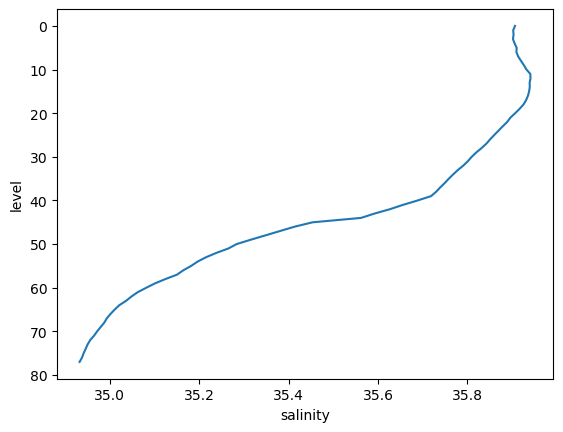
* level (level) int64 0 1 2 3 4 5 6 7 8 9 ... 68 69 70 71 72 73 74 75 76 77However, rather than performing reductions on axes (as in numpy), we can perform them on dimensions. This turns out to be a huge convenience
argo_mean = argo.mean(dim='date')
argo_mean
<xarray.Dataset>
Dimensions: (level: 78)
Coordinates:
* level (level) int64 0 1 2 3 4 5 6 7 8 ... 69 70 71 72 73 74 75 76 77
Data variables:
salinity (level) float64 35.91 35.9 35.9 35.9 ... 34.94 34.94 34.93
temperature (level) float64 17.6 17.57 17.51 17.42 ... 3.789 3.73 3.662
pressure (level) float64 6.435 10.57 15.54 ... 1.95e+03 1.999e+03argo_mean.salinity.plot(y='level', yincrease=False)
[<matplotlib.lines.Line2D at 0x706ffd571d90>]
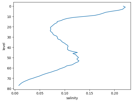
argo_std = argo.std(dim='date')
argo_std.salinity.plot(y='level', yincrease=False)
[<matplotlib.lines.Line2D at 0x706ffd63cbd0>]
20.5.1. Weighted Reductions#
Sometimes we want to perform a reduction (e.g. a mean) where we assign different weight factors to each point in the array.
Xarray supports this via weighted array reductions.
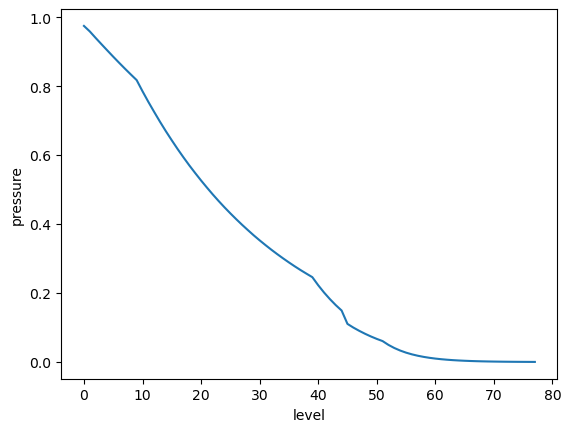
As a toy example, imagine we want to weight values in the upper ocean more than the lower ocean. We could imagine creating a weight array exponentially proportional to pressure as follows:
mean_pressure = argo.pressure.mean(dim='date')
p0 = 250
weights = np.exp(-mean_pressure / p0)
weights.plot()
[<matplotlib.lines.Line2D at 0x706ffd651050>]
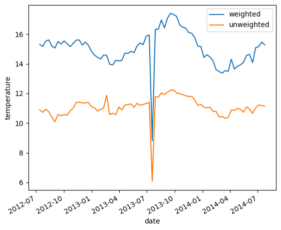
The weighted mean over the level dimensions is calculated as follows:
temp_weighted_mean = argo.temperature.weighted(weights).mean(dim='level')
Comparing to the unweighted mean, we see the difference:
temp_weighted_mean.plot(label='weighted')
argo.temperature.mean(dim='level').plot(label='unweighted')
plt.legend()
<matplotlib.legend.Legend at 0x706ffd3dc210>
20.6. Loading Data from netCDF Files#
NetCDF (Network Common Data Format) is the most widely used format for distributing geoscience data. NetCDF is maintained by the Unidata organization.
Below we quote from the NetCDF website:
NetCDF (network Common Data Form) is a set of interfaces for array-oriented data access and a freely distributed collection of data access libraries for C, Fortran, C++, Java, and other languages. The netCDF libraries support a machine-independent format for representing scientific data. Together, the interfaces, libraries, and format support the creation, access, and sharing of scientific data.
NetCDF data is:
Self-Describing. A netCDF file includes information about the data it contains.
Portable. A netCDF file can be accessed by computers with different ways of storing integers, characters, and floating-point numbers.
Scalable. A small subset of a large dataset may be accessed efficiently.
Appendable. Data may be appended to a properly structured netCDF file without copying the dataset or redefining its structure.
Sharable. One writer and multiple readers may simultaneously access the same netCDF file.
Archivable. Access to all earlier forms of netCDF data will be supported by current and future versions of the software.
Xarray was designed to make reading netCDF files in python as easy, powerful, and flexible as possible. (See xarray netCDF docs for more details.)
Below we download and load some the NASA GISSTemp global temperature anomaly dataset.
gistemp_file = pooch.retrieve(
'https://data.giss.nasa.gov/pub/gistemp/gistemp1200_GHCNv4_ERSSTv5.nc.gz',
known_hash=None,
processor=pooch.Decompress(),
)
ds = xr.open_dataset(gistemp_file)
ds
<xarray.Dataset>
Dimensions: (lat: 90, lon: 180, time: 1725, nv: 2)
Coordinates:
* lat (lat) float32 -89.0 -87.0 -85.0 -83.0 ... 83.0 85.0 87.0 89.0
* lon (lon) float32 -179.0 -177.0 -175.0 -173.0 ... 175.0 177.0 179.0
* time (time) datetime64[ns] 1880-01-15 1880-02-15 ... 2023-09-15
Dimensions without coordinates: nv
Data variables:
time_bnds (time, nv) datetime64[ns] ...
tempanomaly (time, lat, lon) float32 ...
Attributes:
title: GISTEMP Surface Temperature Analysis
institution: NASA Goddard Institute for Space Studies
source: http://data.giss.nasa.gov/gistemp/
Conventions: CF-1.6
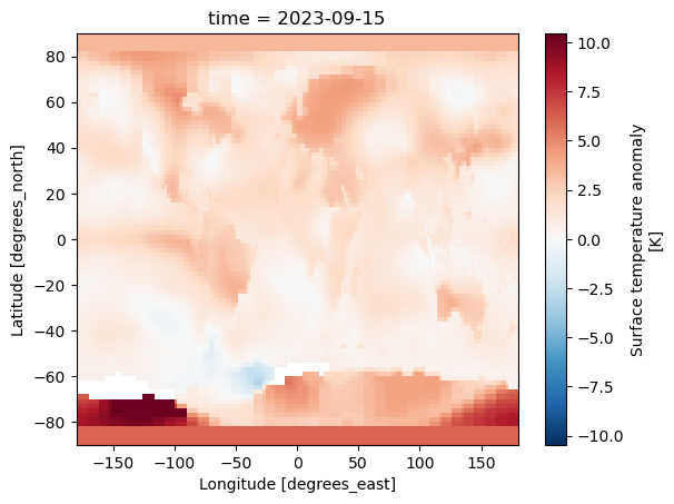
history: Created 2023-10-11 11:54:46 by SBBX_to_nc 2.0 - ILAND=1200,...ds.tempanomaly.isel(time=-1).plot()
<matplotlib.collections.QuadMesh at 0x706ff0312f50>
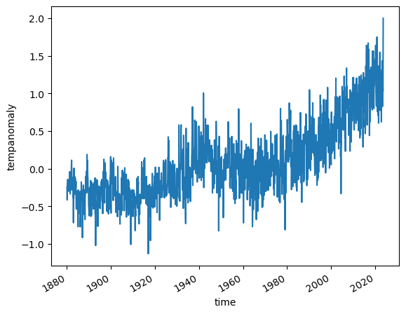
ds.tempanomaly.mean(dim=('lon', 'lat')).plot()
[<matplotlib.lines.Line2D at 0x706ff02b8e50>]
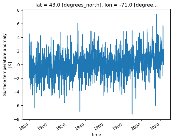
Let’s visualize the temperature anomally for the grid near Worcester. (Worcester’s coordinates: latitude: 42.2626; longtitude: -71.8023)
ds.tempanomaly.sel(lat=42.2626, lon=-71.8023, method='nearest').plot()
[<matplotlib.lines.Line2D at 0x706fe128f610>]
Note that you need to define method since the corresponding values for Worcester latitude and longitude do not exist in the DataArray’s coordinates.