12. Working with CRS and Projections in Python#
The goal of this lecture is to work with PyProj, Cartopy and Shapely packages in Python and explore different crs formats. We will also transform data from one projection to another one.
Attribution: Parts of this notebook is developed using great resources from CLEX CMS Blog and Projection Tradeoffs and Distortion - Tissot
import matplotlib.pyplot as plt
import matplotlib.ticker as mticker
import cartopy.crs as ccrs
import pyproj
import shapely
import leafmap
#Turn off warnings from cartopy
import warnings
warnings.filterwarnings('ignore')
12.1. Convert CRS from one format to the other#
You can generate a crs using caropy’s crs module. For example:
[ccrs.Mercator()]
[<Projected CRS: +proj=merc +ellps=WGS84 +lon_0=0.0 +x_0=0.0 +y_0=0 ...>
 Name: unknown
 Axis Info [cartesian]:
 - E[east]: Easting (metre)
 - N[north]: Northing (metre)
 Area of Use:
 - undefined
 Coordinate Operation:
 - name: unknown
 - method: Mercator (variant A)
 Datum: Unknown based on WGS 84 ellipsoid
 - Ellipsoid: WGS 84
 - Prime Meridian: Greenwich]
ccrs.Mercator()
<cartopy.crs.Mercator object at 0x7f1cbc19e810>
Similarly, you can use pyproj to generate a crs
pyproj.CRS(4326)
<Geographic 2D CRS: EPSG:4326>
Name: WGS 84
Axis Info [ellipsoidal]:
- Lat[north]: Geodetic latitude (degree)
- Lon[east]: Geodetic longitude (degree)
Area of Use:
- name: World.
- bounds: (-180.0, -90.0, 180.0, 90.0)
Datum: World Geodetic System 1984 ensemble
- Ellipsoid: WGS 84
- Prime Meridian: Greenwich
You can use built in function in both pyproj and cartopy to conver the crs between different formats
pyproj.CRS(ccrs.Mercator().to_proj4()).to_epsg()
3395
pyproj.CRS(ccrs.Mercator().to_proj4()).to_wkt()
'PROJCRS["unknown",BASEGEOGCRS["unknown",DATUM["Unknown based on WGS 84 ellipsoid",ELLIPSOID["WGS 84",6378137,298.257223563,LENGTHUNIT["metre",1],ID["EPSG",7030]]],PRIMEM["Greenwich",0,ANGLEUNIT["degree",0.0174532925199433],ID["EPSG",8901]]],CONVERSION["unknown",METHOD["Mercator (variant A)",ID["EPSG",9804]],PARAMETER["Latitude of natural origin",0,ANGLEUNIT["degree",0.0174532925199433],ID["EPSG",8801]],PARAMETER["Longitude of natural origin",0,ANGLEUNIT["degree",0.0174532925199433],ID["EPSG",8802]],PARAMETER["Scale factor at natural origin",1,SCALEUNIT["unity",1],ID["EPSG",8805]],PARAMETER["False easting",0,LENGTHUNIT["metre",1],ID["EPSG",8806]],PARAMETER["False northing",0,LENGTHUNIT["metre",1],ID["EPSG",8807]]],CS[Cartesian,2],AXIS["(E)",east,ORDER[1],LENGTHUNIT["metre",1,ID["EPSG",9001]]],AXIS["(N)",north,ORDER[2],LENGTHUNIT["metre",1,ID["EPSG",9001]]]]'
pyproj.CRS("World_Mercator")
<Projected CRS: ESRI:54004>
Name: World_Mercator
Axis Info [cartesian]:
- E[east]: Easting (metre)
- N[north]: Northing (metre)
Area of Use:
- name: World.
- bounds: (-180.0, -90.0, 180.0, 90.0)
Coordinate Operation:
- name: World_Mercator
- method: Mercator (variant B)
Datum: World Geodetic System 1984 ensemble
- Ellipsoid: WGS 84
- Prime Meridian: Greenwich
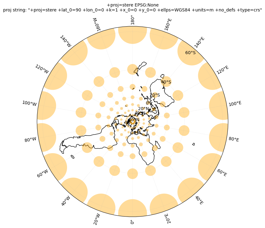
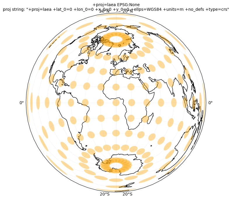
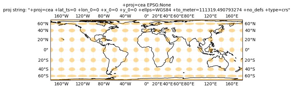
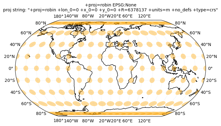
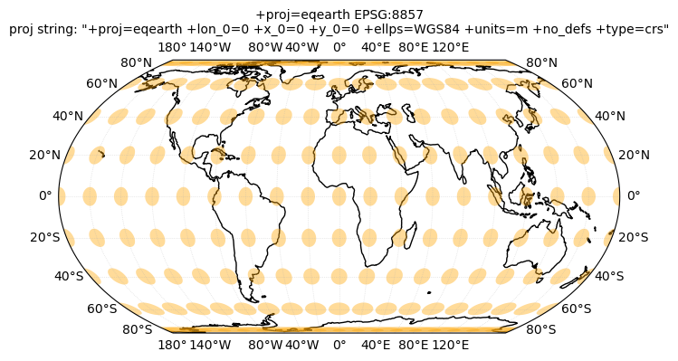
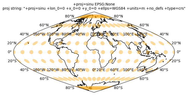
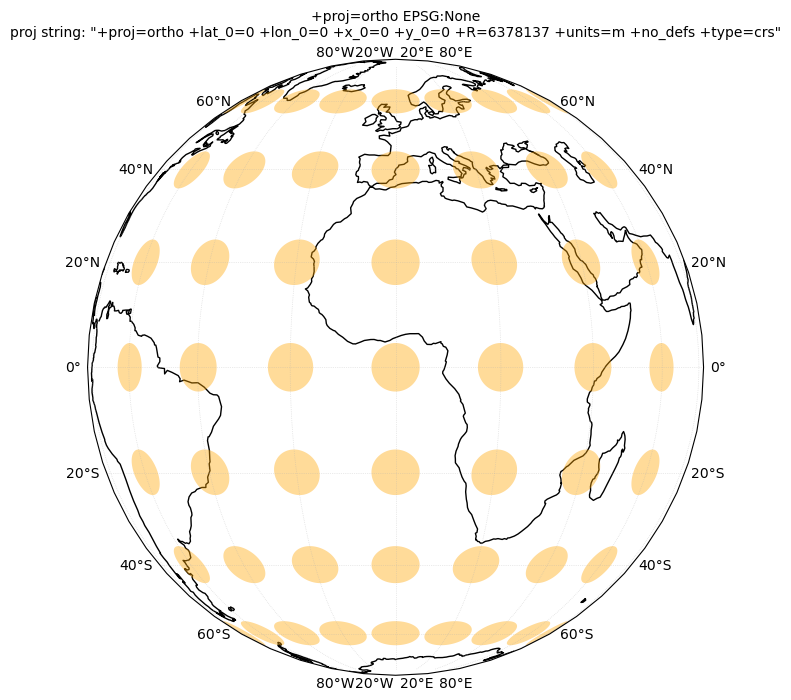
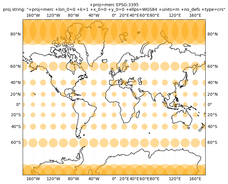
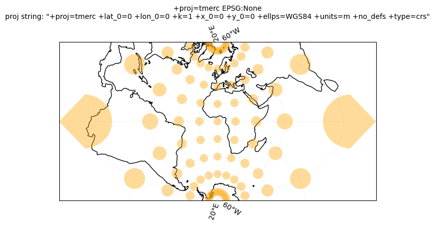
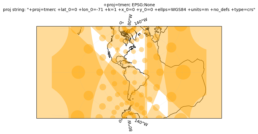
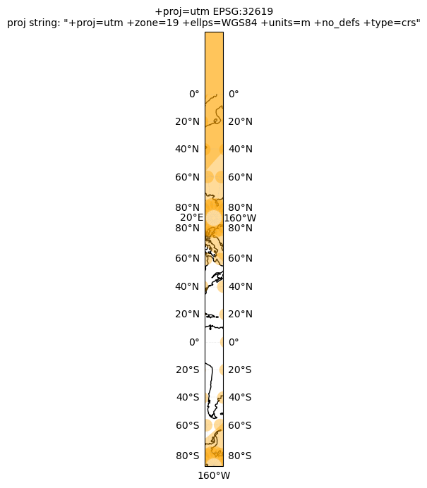
12.2. Tissot’s indicatrix#
Next, we will plot Tissot’s indicatrix for several projections and study map distortions:
#Function to create cartopy plot with Tissot circles for input crs
def tissotplot(crs):

    #Create figure and axes
    fig, ax = plt.subplots(subplot_kw={'projection': crs}, figsize=(8,8))

    #Define positions of the circles, spaced every 20 degrees
    lons = range(-180, 180, 20)
    #lats = range(-90, 90, 20)
    lats = range(-80, 81, 20)

    #Draw coastlines
    ax.coastlines()

    #Add gridlines
    gl = ax.gridlines(draw_labels=True, auto_inline=True, alpha=0.5, lw=0.5, linestyle=':')
    gl.xlocator = mticker.FixedLocator(lons)
    gl.ylocator = mticker.FixedLocator(lats)

    #Add tissot circles with 500 km radius
    ax.tissot(facecolor='orange', alpha=0.4, rad_km=500, lons=lons, lats=lats)

    #Title including projection name and proj string
    crs_name = str(crs).split(' ')[0].split('.')[-1]
    ax.set_title('%s EPSG:%s\nproj string: "%s"' % (crs_name, crs.to_epsg(), crs.to_proj4()), fontsize=10)
#Define projecitons to plot
#Full list is here: https://scitools.org.uk/cartopy/docs/latest/crs/projections.html
crs_list = [ccrs.NorthPolarStereo(), ccrs.LambertAzimuthalEqualArea(), ccrs.LambertCylindrical(), ccrs.Robinson(), \
            ccrs.EqualEarth(), ccrs.Sinusoidal(), ccrs.Orthographic(), ccrs.Mercator(), \
            ccrs.TransverseMercator(), ccrs.TransverseMercator(central_longitude=-71), ccrs.UTM(19)]
for crs in crs_list:
    tissotplot(crs);
12.3. Converting coordinates with Pyproj#
In this part, we will donwload a sample scene of Sentinel-2, and work with its coordinates.
donwload a scene load its coordinates. convert to 4326 plot the coordinates from both CRS
from pystac_client import Client
client = Client.open("https://earth-search.aws.element84.com/v1")
search_results = client.search(
    ids = ["S2B_37DFA_20230224_0_L2A"]
)
items = search_results.item_collection()
item = items[0]
Let’s find the CRS of this scene. The crs is recorded as EPSG numbers in the properties of the item:
item.properties["proj:epsg"]
32737
item
Item: S2B_37DFA_20230224_0_L2A
| id: S2B_37DFA_20230224_0_L2A |
| bbox: [41.77852765935361, -72.16491345575483, 45.122130956889094, -71.11191009560223] |
| created: 2023-02-24T15:02:57.019Z |
| platform: sentinel-2b |
| constellation: sentinel-2 |
| instruments: ['msi'] |
| eo:cloud_cover: 3.506481 |
| proj:epsg: 32737 |
| mgrs:utm_zone: 37 |
| mgrs:latitude_band: D |
| mgrs:grid_square: FA |
| grid:code: MGRS-37DFA |
| view:sun_azimuth: 59.0360301652208 |
| view:sun_elevation: 19.6086887014133 |
| s2:degraded_msi_data_percentage: 0.0131 |
| s2:nodata_pixel_percentage: 0 |
| s2:saturated_defective_pixel_percentage: 0 |
| s2:dark_features_percentage: 0 |
| s2:cloud_shadow_percentage: 0 |
| s2:vegetation_percentage: 0 |
| s2:not_vegetated_percentage: 0 |
| s2:water_percentage: 0 |
| s2:unclassified_percentage: 0 |
| s2:medium_proba_clouds_percentage: 3.506481 |
| s2:high_proba_clouds_percentage: 0 |
| s2:thin_cirrus_percentage: 0 |
| s2:snow_ice_percentage: 96.493524 |
| s2:product_type: S2MSI2A |
| s2:processing_baseline: 05.09 |
| s2:product_uri: S2B_MSIL2A_20230224T053709_N0509_R119_T37DFA_20230224T080819.SAFE |
| s2:generation_time: 2023-02-24T08:08:19.000000Z |
| s2:datatake_id: GS2B_20230224T053709_031176_N05.09 |
| s2:datatake_type: INS-NOBS |
| s2:datastrip_id: S2B_OPER_MSI_L2A_DS_2BPS_20230224T080819_S20230224T053712_N05.09 |
| s2:granule_id: S2B_OPER_MSI_L2A_TL_2BPS_20230224T080819_A031176_T37DFA_N05.09 |
| s2:reflectance_conversion_factor: 1.0232011735908 |
| datetime: 2023-02-24T05:39:35.836000Z |
| s2:sequence: 0 |
| earthsearch:s3_path: s3://sentinel-cogs/sentinel-s2-l2a-cogs/37/D/FA/2023/2/S2B_37DFA_20230224_0_L2A |
| earthsearch:payload_id: roda-sentinel2/workflow-sentinel2-to-stac/9a7e8b645adfa65d16b5e5a19d43d598 |
| earthsearch:boa_offset_applied: True |
| processing:software: {'sentinel2-to-stac': '0.1.0'} |
| updated: 2023-02-24T15:02:57.019Z |
STAC Extensions
Assets
Asset: Aerosol optical thickness (AOT)
| href: https://sentinel-cogs.s3.us-west-2.amazonaws.com/sentinel-s2-l2a-cogs/37/D/FA/2023/2/S2B_37DFA_20230224_0_L2A/AOT.tif |
| type: image/tiff; application=geotiff; profile=cloud-optimized |
| title: Aerosol optical thickness (AOT) |
| roles: ['data', 'reflectance'] |
| owner: S2B_37DFA_20230224_0_L2A |
| proj:shape: [5490, 5490] |
| proj:transform: [20, 0, 600000, 0, -20, 2100040] |
| raster:bands: [{'nodata': 0, 'data_type': 'uint16', 'bits_per_sample': 15, 'spatial_resolution': 20, 'scale': 0.001, 'offset': 0}] |
Asset: Blue (band 2) - 10m
| href: https://sentinel-cogs.s3.us-west-2.amazonaws.com/sentinel-s2-l2a-cogs/37/D/FA/2023/2/S2B_37DFA_20230224_0_L2A/B02.tif |
| type: image/tiff; application=geotiff; profile=cloud-optimized |
| title: Blue (band 2) - 10m |
| roles: ['data', 'reflectance'] |
| owner: S2B_37DFA_20230224_0_L2A |
| eo:bands: [{'name': 'blue', 'common_name': 'blue', 'description': 'Blue (band 2)', 'center_wavelength': 0.49, 'full_width_half_max': 0.098}] |
| gsd: 10 |
| proj:shape: [10980, 10980] |
| proj:transform: [10, 0, 600000, 0, -10, 2100040] |
| raster:bands: [{'nodata': 0, 'data_type': 'uint16', 'bits_per_sample': 15, 'spatial_resolution': 10, 'scale': 0.0001, 'offset': -0.1}] |
Asset: Coastal aerosol (band 1) - 60m
| href: https://sentinel-cogs.s3.us-west-2.amazonaws.com/sentinel-s2-l2a-cogs/37/D/FA/2023/2/S2B_37DFA_20230224_0_L2A/B01.tif |
| type: image/tiff; application=geotiff; profile=cloud-optimized |
| title: Coastal aerosol (band 1) - 60m |
| roles: ['data', 'reflectance'] |
| owner: S2B_37DFA_20230224_0_L2A |
| eo:bands: [{'name': 'coastal', 'common_name': 'coastal', 'description': 'Coastal aerosol (band 1)', 'center_wavelength': 0.443, 'full_width_half_max': 0.027}] |
| gsd: 60 |
| proj:shape: [1830, 1830] |
| proj:transform: [60, 0, 600000, 0, -60, 2100040] |
| raster:bands: [{'nodata': 0, 'data_type': 'uint16', 'bits_per_sample': 15, 'spatial_resolution': 60, 'scale': 0.0001, 'offset': -0.1}] |
Asset:
| href: https://sentinel-cogs.s3.us-west-2.amazonaws.com/sentinel-s2-l2a-cogs/37/D/FA/2023/2/S2B_37DFA_20230224_0_L2A/granule_metadata.xml |
| type: application/xml |
| roles: ['metadata'] |
| owner: S2B_37DFA_20230224_0_L2A |
Asset: Green (band 3) - 10m
| href: https://sentinel-cogs.s3.us-west-2.amazonaws.com/sentinel-s2-l2a-cogs/37/D/FA/2023/2/S2B_37DFA_20230224_0_L2A/B03.tif |
| type: image/tiff; application=geotiff; profile=cloud-optimized |
| title: Green (band 3) - 10m |
| roles: ['data', 'reflectance'] |
| owner: S2B_37DFA_20230224_0_L2A |
| eo:bands: [{'name': 'green', 'common_name': 'green', 'description': 'Green (band 3)', 'center_wavelength': 0.56, 'full_width_half_max': 0.045}] |
| gsd: 10 |
| proj:shape: [10980, 10980] |
| proj:transform: [10, 0, 600000, 0, -10, 2100040] |
| raster:bands: [{'nodata': 0, 'data_type': 'uint16', 'bits_per_sample': 15, 'spatial_resolution': 10, 'scale': 0.0001, 'offset': -0.1}] |
Asset: NIR 1 (band 8) - 10m
| href: https://sentinel-cogs.s3.us-west-2.amazonaws.com/sentinel-s2-l2a-cogs/37/D/FA/2023/2/S2B_37DFA_20230224_0_L2A/B08.tif |
| type: image/tiff; application=geotiff; profile=cloud-optimized |
| title: NIR 1 (band 8) - 10m |
| roles: ['data', 'reflectance'] |
| owner: S2B_37DFA_20230224_0_L2A |
| eo:bands: [{'name': 'nir', 'common_name': 'nir', 'description': 'NIR 1 (band 8)', 'center_wavelength': 0.842, 'full_width_half_max': 0.145}] |
| gsd: 10 |
| proj:shape: [10980, 10980] |
| proj:transform: [10, 0, 600000, 0, -10, 2100040] |
| raster:bands: [{'nodata': 0, 'data_type': 'uint16', 'bits_per_sample': 15, 'spatial_resolution': 10, 'scale': 0.0001, 'offset': -0.1}] |
Asset: NIR 2 (band 8A) - 20m
| href: https://sentinel-cogs.s3.us-west-2.amazonaws.com/sentinel-s2-l2a-cogs/37/D/FA/2023/2/S2B_37DFA_20230224_0_L2A/B8A.tif |
| type: image/tiff; application=geotiff; profile=cloud-optimized |
| title: NIR 2 (band 8A) - 20m |
| roles: ['data', 'reflectance'] |
| owner: S2B_37DFA_20230224_0_L2A |
| eo:bands: [{'name': 'nir08', 'common_name': 'nir08', 'description': 'NIR 2 (band 8A)', 'center_wavelength': 0.865, 'full_width_half_max': 0.033}] |
| gsd: 20 |
| proj:shape: [5490, 5490] |
| proj:transform: [20, 0, 600000, 0, -20, 2100040] |
| raster:bands: [{'nodata': 0, 'data_type': 'uint16', 'bits_per_sample': 15, 'spatial_resolution': 20, 'scale': 0.0001, 'offset': -0.1}] |
Asset: NIR 3 (band 9) - 60m
| href: https://sentinel-cogs.s3.us-west-2.amazonaws.com/sentinel-s2-l2a-cogs/37/D/FA/2023/2/S2B_37DFA_20230224_0_L2A/B09.tif |
| type: image/tiff; application=geotiff; profile=cloud-optimized |
| title: NIR 3 (band 9) - 60m |
| roles: ['data', 'reflectance'] |
| owner: S2B_37DFA_20230224_0_L2A |
| eo:bands: [{'name': 'nir09', 'common_name': 'nir09', 'description': 'NIR 3 (band 9)', 'center_wavelength': 0.945, 'full_width_half_max': 0.026}] |
| gsd: 60 |
| proj:shape: [1830, 1830] |
| proj:transform: [60, 0, 600000, 0, -60, 2100040] |
| raster:bands: [{'nodata': 0, 'data_type': 'uint16', 'bits_per_sample': 15, 'spatial_resolution': 60, 'scale': 0.0001, 'offset': -0.1}] |
Asset: Red (band 4) - 10m
| href: https://sentinel-cogs.s3.us-west-2.amazonaws.com/sentinel-s2-l2a-cogs/37/D/FA/2023/2/S2B_37DFA_20230224_0_L2A/B04.tif |
| type: image/tiff; application=geotiff; profile=cloud-optimized |
| title: Red (band 4) - 10m |
| roles: ['data', 'reflectance'] |
| owner: S2B_37DFA_20230224_0_L2A |
| eo:bands: [{'name': 'red', 'common_name': 'red', 'description': 'Red (band 4)', 'center_wavelength': 0.665, 'full_width_half_max': 0.038}] |
| gsd: 10 |
| proj:shape: [10980, 10980] |
| proj:transform: [10, 0, 600000, 0, -10, 2100040] |
| raster:bands: [{'nodata': 0, 'data_type': 'uint16', 'bits_per_sample': 15, 'spatial_resolution': 10, 'scale': 0.0001, 'offset': -0.1}] |
Asset: Red edge 1 (band 5) - 20m
| href: https://sentinel-cogs.s3.us-west-2.amazonaws.com/sentinel-s2-l2a-cogs/37/D/FA/2023/2/S2B_37DFA_20230224_0_L2A/B05.tif |
| type: image/tiff; application=geotiff; profile=cloud-optimized |
| title: Red edge 1 (band 5) - 20m |
| roles: ['data', 'reflectance'] |
| owner: S2B_37DFA_20230224_0_L2A |
| eo:bands: [{'name': 'rededge1', 'common_name': 'rededge', 'description': 'Red edge 1 (band 5)', 'center_wavelength': 0.704, 'full_width_half_max': 0.019}] |
| gsd: 20 |
| proj:shape: [5490, 5490] |
| proj:transform: [20, 0, 600000, 0, -20, 2100040] |
| raster:bands: [{'nodata': 0, 'data_type': 'uint16', 'bits_per_sample': 15, 'spatial_resolution': 20, 'scale': 0.0001, 'offset': -0.1}] |
Asset: Red edge 2 (band 6) - 20m
| href: https://sentinel-cogs.s3.us-west-2.amazonaws.com/sentinel-s2-l2a-cogs/37/D/FA/2023/2/S2B_37DFA_20230224_0_L2A/B06.tif |
| type: image/tiff; application=geotiff; profile=cloud-optimized |
| title: Red edge 2 (band 6) - 20m |
| roles: ['data', 'reflectance'] |
| owner: S2B_37DFA_20230224_0_L2A |
| eo:bands: [{'name': 'rededge2', 'common_name': 'rededge', 'description': 'Red edge 2 (band 6)', 'center_wavelength': 0.74, 'full_width_half_max': 0.018}] |
| gsd: 20 |
| proj:shape: [5490, 5490] |
| proj:transform: [20, 0, 600000, 0, -20, 2100040] |
| raster:bands: [{'nodata': 0, 'data_type': 'uint16', 'bits_per_sample': 15, 'spatial_resolution': 20, 'scale': 0.0001, 'offset': -0.1}] |
Asset: Red edge 3 (band 7) - 20m
| href: https://sentinel-cogs.s3.us-west-2.amazonaws.com/sentinel-s2-l2a-cogs/37/D/FA/2023/2/S2B_37DFA_20230224_0_L2A/B07.tif |
| type: image/tiff; application=geotiff; profile=cloud-optimized |
| title: Red edge 3 (band 7) - 20m |
| roles: ['data', 'reflectance'] |
| owner: S2B_37DFA_20230224_0_L2A |
| eo:bands: [{'name': 'rededge3', 'common_name': 'rededge', 'description': 'Red edge 3 (band 7)', 'center_wavelength': 0.783, 'full_width_half_max': 0.028}] |
| gsd: 20 |
| proj:shape: [5490, 5490] |
| proj:transform: [20, 0, 600000, 0, -20, 2100040] |
| raster:bands: [{'nodata': 0, 'data_type': 'uint16', 'bits_per_sample': 15, 'spatial_resolution': 20, 'scale': 0.0001, 'offset': -0.1}] |
Asset: Scene classification map (SCL)
| href: https://sentinel-cogs.s3.us-west-2.amazonaws.com/sentinel-s2-l2a-cogs/37/D/FA/2023/2/S2B_37DFA_20230224_0_L2A/SCL.tif |
| type: image/tiff; application=geotiff; profile=cloud-optimized |
| title: Scene classification map (SCL) |
| roles: ['data', 'reflectance'] |
| owner: S2B_37DFA_20230224_0_L2A |
| proj:shape: [5490, 5490] |
| proj:transform: [20, 0, 600000, 0, -20, 2100040] |
| raster:bands: [{'nodata': 0, 'data_type': 'uint8', 'spatial_resolution': 20}] |
Asset: SWIR 1 (band 11) - 20m
| href: https://sentinel-cogs.s3.us-west-2.amazonaws.com/sentinel-s2-l2a-cogs/37/D/FA/2023/2/S2B_37DFA_20230224_0_L2A/B11.tif |
| type: image/tiff; application=geotiff; profile=cloud-optimized |
| title: SWIR 1 (band 11) - 20m |
| roles: ['data', 'reflectance'] |
| owner: S2B_37DFA_20230224_0_L2A |
| eo:bands: [{'name': 'swir16', 'common_name': 'swir16', 'description': 'SWIR 1 (band 11)', 'center_wavelength': 1.61, 'full_width_half_max': 0.143}] |
| gsd: 20 |
| proj:shape: [5490, 5490] |
| proj:transform: [20, 0, 600000, 0, -20, 2100040] |
| raster:bands: [{'nodata': 0, 'data_type': 'uint16', 'bits_per_sample': 15, 'spatial_resolution': 20, 'scale': 0.0001, 'offset': -0.1}] |
Asset: SWIR 2 (band 12) - 20m
| href: https://sentinel-cogs.s3.us-west-2.amazonaws.com/sentinel-s2-l2a-cogs/37/D/FA/2023/2/S2B_37DFA_20230224_0_L2A/B12.tif |
| type: image/tiff; application=geotiff; profile=cloud-optimized |
| title: SWIR 2 (band 12) - 20m |
| roles: ['data', 'reflectance'] |
| owner: S2B_37DFA_20230224_0_L2A |
| eo:bands: [{'name': 'swir22', 'common_name': 'swir22', 'description': 'SWIR 2 (band 12)', 'center_wavelength': 2.19, 'full_width_half_max': 0.242}] |
| gsd: 20 |
| proj:shape: [5490, 5490] |
| proj:transform: [20, 0, 600000, 0, -20, 2100040] |
| raster:bands: [{'nodata': 0, 'data_type': 'uint16', 'bits_per_sample': 15, 'spatial_resolution': 20, 'scale': 0.0001, 'offset': -0.1}] |
Asset: Thumbnail image
| href: https://sentinel-cogs.s3.us-west-2.amazonaws.com/sentinel-s2-l2a-cogs/37/D/FA/2023/2/S2B_37DFA_20230224_0_L2A/thumbnail.jpg |
| type: image/jpeg |
| title: Thumbnail image |
| roles: ['thumbnail'] |
| owner: S2B_37DFA_20230224_0_L2A |
Asset:
| href: https://sentinel-cogs.s3.us-west-2.amazonaws.com/sentinel-s2-l2a-cogs/37/D/FA/2023/2/S2B_37DFA_20230224_0_L2A/tileinfo_metadata.json |
| type: application/json |
| roles: ['metadata'] |
| owner: S2B_37DFA_20230224_0_L2A |
Asset: True color image
| href: https://sentinel-cogs.s3.us-west-2.amazonaws.com/sentinel-s2-l2a-cogs/37/D/FA/2023/2/S2B_37DFA_20230224_0_L2A/TCI.tif |
| type: image/tiff; application=geotiff; profile=cloud-optimized |
| title: True color image |
| roles: ['visual'] |
| owner: S2B_37DFA_20230224_0_L2A |
| eo:bands: [{'name': 'red', 'common_name': 'red', 'description': 'Red (band 4)', 'center_wavelength': 0.665, 'full_width_half_max': 0.038}, {'name': 'green', 'common_name': 'green', 'description': 'Green (band 3)', 'center_wavelength': 0.56, 'full_width_half_max': 0.045}, {'name': 'blue', 'common_name': 'blue', 'description': 'Blue (band 2)', 'center_wavelength': 0.49, 'full_width_half_max': 0.098}] |
| proj:shape: [10980, 10980] |
| proj:transform: [10, 0, 600000, 0, -10, 2100040] |
Asset: Water vapour (WVP)
| href: https://sentinel-cogs.s3.us-west-2.amazonaws.com/sentinel-s2-l2a-cogs/37/D/FA/2023/2/S2B_37DFA_20230224_0_L2A/WVP.tif |
| type: image/tiff; application=geotiff; profile=cloud-optimized |
| title: Water vapour (WVP) |
| roles: ['data', 'reflectance'] |
| owner: S2B_37DFA_20230224_0_L2A |
| proj:shape: [5490, 5490] |
| proj:transform: [20, 0, 600000, 0, -20, 2100040] |
| raster:bands: [{'nodata': 0, 'data_type': 'uint16', 'bits_per_sample': 15, 'spatial_resolution': 20, 'unit': 'cm', 'scale': 0.001, 'offset': 0}] |
Asset: Aerosol optical thickness (AOT)
| href: s3://sentinel-s2-l2a/tiles/37/D/FA/2023/2/24/0/AOT.jp2 |
| type: image/jp2 |
| title: Aerosol optical thickness (AOT) |
| roles: ['data', 'reflectance'] |
| owner: S2B_37DFA_20230224_0_L2A |
| proj:shape: [5490, 5490] |
| proj:transform: [20, 0, 600000, 0, -20, 2100040] |
| raster:bands: [{'nodata': 0, 'data_type': 'uint16', 'bits_per_sample': 15, 'spatial_resolution': 20, 'scale': 0.001, 'offset': 0}] |
Asset: Blue (band 2) - 10m
| href: s3://sentinel-s2-l2a/tiles/37/D/FA/2023/2/24/0/B02.jp2 |
| type: image/jp2 |
| title: Blue (band 2) - 10m |
| roles: ['data', 'reflectance'] |
| owner: S2B_37DFA_20230224_0_L2A |
| eo:bands: [{'name': 'blue', 'common_name': 'blue', 'description': 'Blue (band 2)', 'center_wavelength': 0.49, 'full_width_half_max': 0.098}] |
| gsd: 10 |
| proj:shape: [10980, 10980] |
| proj:transform: [10, 0, 600000, 0, -10, 2100040] |
| raster:bands: [{'nodata': 0, 'data_type': 'uint16', 'bits_per_sample': 15, 'spatial_resolution': 10, 'scale': 0.0001, 'offset': -0.1}] |
Asset: Coastal aerosol (band 1) - 60m
| href: s3://sentinel-s2-l2a/tiles/37/D/FA/2023/2/24/0/B01.jp2 |
| type: image/jp2 |
| title: Coastal aerosol (band 1) - 60m |
| roles: ['data', 'reflectance'] |
| owner: S2B_37DFA_20230224_0_L2A |
| eo:bands: [{'name': 'coastal', 'common_name': 'coastal', 'description': 'Coastal aerosol (band 1)', 'center_wavelength': 0.443, 'full_width_half_max': 0.027}] |
| gsd: 60 |
| proj:shape: [1830, 1830] |
| proj:transform: [60, 0, 600000, 0, -60, 2100040] |
| raster:bands: [{'nodata': 0, 'data_type': 'uint16', 'bits_per_sample': 15, 'spatial_resolution': 60, 'scale': 0.0001, 'offset': -0.1}] |
Asset: Green (band 3) - 10m
| href: s3://sentinel-s2-l2a/tiles/37/D/FA/2023/2/24/0/B03.jp2 |
| type: image/jp2 |
| title: Green (band 3) - 10m |
| roles: ['data', 'reflectance'] |
| owner: S2B_37DFA_20230224_0_L2A |
| eo:bands: [{'name': 'green', 'common_name': 'green', 'description': 'Green (band 3)', 'center_wavelength': 0.56, 'full_width_half_max': 0.045}] |
| gsd: 10 |
| proj:shape: [10980, 10980] |
| proj:transform: [10, 0, 600000, 0, -10, 2100040] |
| raster:bands: [{'nodata': 0, 'data_type': 'uint16', 'bits_per_sample': 15, 'spatial_resolution': 10, 'scale': 0.0001, 'offset': -0.1}] |
Asset: NIR 1 (band 8) - 10m
| href: s3://sentinel-s2-l2a/tiles/37/D/FA/2023/2/24/0/B08.jp2 |
| type: image/jp2 |
| title: NIR 1 (band 8) - 10m |
| roles: ['data', 'reflectance'] |
| owner: S2B_37DFA_20230224_0_L2A |
| eo:bands: [{'name': 'nir', 'common_name': 'nir', 'description': 'NIR 1 (band 8)', 'center_wavelength': 0.842, 'full_width_half_max': 0.145}] |
| gsd: 10 |
| proj:shape: [10980, 10980] |
| proj:transform: [10, 0, 600000, 0, -10, 2100040] |
| raster:bands: [{'nodata': 0, 'data_type': 'uint16', 'bits_per_sample': 15, 'spatial_resolution': 10, 'scale': 0.0001, 'offset': -0.1}] |
Asset: NIR 2 (band 8A) - 20m
| href: s3://sentinel-s2-l2a/tiles/37/D/FA/2023/2/24/0/B8A.jp2 |
| type: image/jp2 |
| title: NIR 2 (band 8A) - 20m |
| roles: ['data', 'reflectance'] |
| owner: S2B_37DFA_20230224_0_L2A |
| eo:bands: [{'name': 'nir08', 'common_name': 'nir08', 'description': 'NIR 2 (band 8A)', 'center_wavelength': 0.865, 'full_width_half_max': 0.033}] |
| gsd: 20 |
| proj:shape: [5490, 5490] |
| proj:transform: [20, 0, 600000, 0, -20, 2100040] |
| raster:bands: [{'nodata': 0, 'data_type': 'uint16', 'bits_per_sample': 15, 'spatial_resolution': 20, 'scale': 0.0001, 'offset': -0.1}] |
Asset: NIR 3 (band 9) - 60m
| href: s3://sentinel-s2-l2a/tiles/37/D/FA/2023/2/24/0/B09.jp2 |
| type: image/jp2 |
| title: NIR 3 (band 9) - 60m |
| roles: ['data', 'reflectance'] |
| owner: S2B_37DFA_20230224_0_L2A |
| eo:bands: [{'name': 'nir09', 'common_name': 'nir09', 'description': 'NIR 3 (band 9)', 'center_wavelength': 0.945, 'full_width_half_max': 0.026}] |
| gsd: 60 |
| proj:shape: [1830, 1830] |
| proj:transform: [60, 0, 600000, 0, -60, 2100040] |
| raster:bands: [{'nodata': 0, 'data_type': 'uint16', 'bits_per_sample': 15, 'spatial_resolution': 60, 'scale': 0.0001, 'offset': -0.1}] |
Asset: Red (band 4) - 10m
| href: s3://sentinel-s2-l2a/tiles/37/D/FA/2023/2/24/0/B04.jp2 |
| type: image/jp2 |
| title: Red (band 4) - 10m |
| roles: ['data', 'reflectance'] |
| owner: S2B_37DFA_20230224_0_L2A |
| eo:bands: [{'name': 'red', 'common_name': 'red', 'description': 'Red (band 4)', 'center_wavelength': 0.665, 'full_width_half_max': 0.038}] |
| gsd: 10 |
| proj:shape: [10980, 10980] |
| proj:transform: [10, 0, 600000, 0, -10, 2100040] |
| raster:bands: [{'nodata': 0, 'data_type': 'uint16', 'bits_per_sample': 15, 'spatial_resolution': 10, 'scale': 0.0001, 'offset': -0.1}] |
Asset: Red edge 1 (band 5) - 20m
| href: s3://sentinel-s2-l2a/tiles/37/D/FA/2023/2/24/0/B05.jp2 |
| type: image/jp2 |
| title: Red edge 1 (band 5) - 20m |
| roles: ['data', 'reflectance'] |
| owner: S2B_37DFA_20230224_0_L2A |
| eo:bands: [{'name': 'rededge1', 'common_name': 'rededge', 'description': 'Red edge 1 (band 5)', 'center_wavelength': 0.704, 'full_width_half_max': 0.019}] |
| gsd: 20 |
| proj:shape: [5490, 5490] |
| proj:transform: [20, 0, 600000, 0, -20, 2100040] |
| raster:bands: [{'nodata': 0, 'data_type': 'uint16', 'bits_per_sample': 15, 'spatial_resolution': 20, 'scale': 0.0001, 'offset': -0.1}] |
Asset: Red edge 2 (band 6) - 20m
| href: s3://sentinel-s2-l2a/tiles/37/D/FA/2023/2/24/0/B06.jp2 |
| type: image/jp2 |
| title: Red edge 2 (band 6) - 20m |
| roles: ['data', 'reflectance'] |
| owner: S2B_37DFA_20230224_0_L2A |
| eo:bands: [{'name': 'rededge2', 'common_name': 'rededge', 'description': 'Red edge 2 (band 6)', 'center_wavelength': 0.74, 'full_width_half_max': 0.018}] |
| gsd: 20 |
| proj:shape: [5490, 5490] |
| proj:transform: [20, 0, 600000, 0, -20, 2100040] |
| raster:bands: [{'nodata': 0, 'data_type': 'uint16', 'bits_per_sample': 15, 'spatial_resolution': 20, 'scale': 0.0001, 'offset': -0.1}] |
Asset: Red edge 3 (band 7) - 20m
| href: s3://sentinel-s2-l2a/tiles/37/D/FA/2023/2/24/0/B07.jp2 |
| type: image/jp2 |
| title: Red edge 3 (band 7) - 20m |
| roles: ['data', 'reflectance'] |
| owner: S2B_37DFA_20230224_0_L2A |
| eo:bands: [{'name': 'rededge3', 'common_name': 'rededge', 'description': 'Red edge 3 (band 7)', 'center_wavelength': 0.783, 'full_width_half_max': 0.028}] |
| gsd: 20 |
| proj:shape: [5490, 5490] |
| proj:transform: [20, 0, 600000, 0, -20, 2100040] |
| raster:bands: [{'nodata': 0, 'data_type': 'uint16', 'bits_per_sample': 15, 'spatial_resolution': 20, 'scale': 0.0001, 'offset': -0.1}] |
Asset: Scene classification map (SCL)
| href: s3://sentinel-s2-l2a/tiles/37/D/FA/2023/2/24/0/SCL.jp2 |
| type: image/jp2 |
| title: Scene classification map (SCL) |
| roles: ['data', 'reflectance'] |
| owner: S2B_37DFA_20230224_0_L2A |
| proj:shape: [5490, 5490] |
| proj:transform: [20, 0, 600000, 0, -20, 2100040] |
| raster:bands: [{'nodata': 0, 'data_type': 'uint8', 'spatial_resolution': 20}] |
Asset: SWIR 1 (band 11) - 20m
| href: s3://sentinel-s2-l2a/tiles/37/D/FA/2023/2/24/0/B11.jp2 |
| type: image/jp2 |
| title: SWIR 1 (band 11) - 20m |
| roles: ['data', 'reflectance'] |
| owner: S2B_37DFA_20230224_0_L2A |
| eo:bands: [{'name': 'swir16', 'common_name': 'swir16', 'description': 'SWIR 1 (band 11)', 'center_wavelength': 1.61, 'full_width_half_max': 0.143}] |
| gsd: 20 |
| proj:shape: [5490, 5490] |
| proj:transform: [20, 0, 600000, 0, -20, 2100040] |
| raster:bands: [{'nodata': 0, 'data_type': 'uint16', 'bits_per_sample': 15, 'spatial_resolution': 20, 'scale': 0.0001, 'offset': -0.1}] |
Asset: SWIR 2 (band 12) - 20m
| href: s3://sentinel-s2-l2a/tiles/37/D/FA/2023/2/24/0/B12.jp2 |
| type: image/jp2 |
| title: SWIR 2 (band 12) - 20m |
| roles: ['data', 'reflectance'] |
| owner: S2B_37DFA_20230224_0_L2A |
| eo:bands: [{'name': 'swir22', 'common_name': 'swir22', 'description': 'SWIR 2 (band 12)', 'center_wavelength': 2.19, 'full_width_half_max': 0.242}] |
| gsd: 20 |
| proj:shape: [5490, 5490] |
| proj:transform: [20, 0, 600000, 0, -20, 2100040] |
| raster:bands: [{'nodata': 0, 'data_type': 'uint16', 'bits_per_sample': 15, 'spatial_resolution': 20, 'scale': 0.0001, 'offset': -0.1}] |
Asset: True color image
| href: s3://sentinel-s2-l2a/tiles/37/D/FA/2023/2/24/0/TCI.jp2 |
| type: image/jp2 |
| title: True color image |
| roles: ['visual'] |
| owner: S2B_37DFA_20230224_0_L2A |
| eo:bands: [{'name': 'red', 'common_name': 'red', 'description': 'Red (band 4)', 'center_wavelength': 0.665, 'full_width_half_max': 0.038}, {'name': 'green', 'common_name': 'green', 'description': 'Green (band 3)', 'center_wavelength': 0.56, 'full_width_half_max': 0.045}, {'name': 'blue', 'common_name': 'blue', 'description': 'Blue (band 2)', 'center_wavelength': 0.49, 'full_width_half_max': 0.098}] |
| proj:shape: [10980, 10980] |
| proj:transform: [10, 0, 600000, 0, -10, 2100040] |
Asset: Water vapour (WVP)
| href: s3://sentinel-s2-l2a/tiles/37/D/FA/2023/2/24/0/WVP.jp2 |
| type: image/jp2 |
| title: Water vapour (WVP) |
| roles: ['data', 'reflectance'] |
| owner: S2B_37DFA_20230224_0_L2A |
| proj:shape: [5490, 5490] |
| proj:transform: [20, 0, 600000, 0, -20, 2100040] |
| raster:bands: [{'nodata': 0, 'data_type': 'uint16', 'bits_per_sample': 15, 'spatial_resolution': 20, 'unit': 'cm', 'scale': 0.001, 'offset': 0}] |
Links
Link:
| rel: self |
| href: https://earth-search.aws.element84.com/v1/collections/sentinel-2-l2a/items/S2B_37DFA_20230224_0_L2A |
| type: application/geo+json |
Link:
| rel: canonical |
| href: s3://sentinel-cogs/sentinel-s2-l2a-cogs/37/D/FA/2023/2/S2B_37DFA_20230224_0_L2A/S2B_37DFA_20230224_0_L2A.json |
| type: application/json |
Link:
| rel: license |
| href: https://sentinel.esa.int/documents/247904/690755/Sentinel_Data_Legal_Notice |
Link:
| rel: derived_from |
| href: https://earth-search.aws.element84.com/v1/collections/sentinel-2-l1c/items/S2B_37DFA_20230224_0_L1C |
| type: application/geo+json |
Link:
| rel: parent |
| href: https://earth-search.aws.element84.com/v1/collections/sentinel-2-l2a |
| type: application/json |
Link:
| rel: collection |
| href: https://earth-search.aws.element84.com/v1/collections/sentinel-2-l2a |
| type: application/json |
Link: Earth Search by Element 84
| rel: root |
| href: https://earth-search.aws.element84.com/v1 |
| type: application/json |
| title: Earth Search by Element 84 |
Link:
| rel: thumbnail |
| href: https://earth-search.aws.element84.com/v1/collections/sentinel-2-l2a/items/S2B_37DFA_20230224_0_L2A/thumbnail |
item.geometry
{'type': 'Polygon',
 'coordinates': [[[41.77852765935361, -71.18173043681364],
   [44.81460295895618, -71.11191009560223],
   [45.122130956889094, -72.09098682450592],
   [41.926326307987814, -72.16491345575483],
   [41.77852765935361, -71.18173043681364]]]}
The STAC metadata contains a geometry for each item. This geometry is recorded in EPSG:4326 (check the specification here). Now, we will convert this from 4326 to the crs of the scene.
To transfrom coordinates from one crs to another one, we will creates a transformer using pyproj, and then input each point to transform it.
source_crs = 'epsg:4326' # Global lat-lon coordinate system used by `geometry m
target_crs = f'epsg:{item.properties["proj:epsg"]}' # Coordinate system of the S-2 scene

latlon_to_s2_transformer = pyproj.Transformer.from_crs(source_crs, target_crs)
Let’s retrieve the geometry from the item metadata:
geometry = item.geometry
geometry
{'type': 'Polygon',
 'coordinates': [[[41.77852765935361, -71.18173043681364],
   [44.81460295895618, -71.11191009560223],
   [45.122130956889094, -72.09098682450592],
   [41.926326307987814, -72.16491345575483],
   [41.77852765935361, -71.18173043681364]]]}
Now, create an empty geometry for our projected geometry:
projected_geometry = {
    "type": "Polygon",
    "coordinates" : [[]]
}
projected_coordinates = []
for point in geometry["coordinates"][0]:
    projected_x, projected_y = latlon_to_s2_transformer.transform(point[0], point[1])
    projected_coordinates.append([projected_x, projected_y])
projected_geometry["coordinates"] = [projected_coordinates]
projected_geometry
{'type': 'Polygon',
 'coordinates': [[[-5034706.161102917, 22347375.738133498],
   [-4631227.676135911, 22123291.71715717],
   [-4542728.576578871, 22192903.107910063],
   [-4958974.741806454, 22435202.22502178],
   [-5034706.161102917, 22347375.738133498]]]}
12.4. Use Shapely to work with geometries#
Another useful Python package, is Shapely for analysis and manipulation of geometric features. Here, we will use it to investigate our geometries. Note that Shapely doesn’t have a notion of crs, and only look at the object as a geomtric object.
Shapely has a reach set of objects, and here we will use the Polygon one. You can create a Shapely Polygon using the following:
shapely_geo = shapely.geometry.shape(geometry)
shapely_geo

Let’s retrieve a property of the this Polygon, such as area:
shapely_geo.bounds
(41.77852765935361, -72.16491345575483, 45.122130956889094, -71.11191009560223)
shapely_geo.area
3.0735047508188207
We can do the same using the projected geometry:
shapely_projected_geo = shapely.geometry.shape(projected_geometry)
shapely_projected_geo

shapely_projected_geo.area
51412513482.37867
As you can see, the areas are very different. In this case, geometry is in lat/lon coordinates, and projected_geometry is in UTM coordinates (meter). Therefore, their corresponding areas are in their native units.
But we can confirm that these two polygons are indeed the same:
First Approach: Tranform the polygon back to its original coordinates:
source_crs = f'epsg:{item.properties["proj:epsg"]}' # Coordinate system of the S-2 scene
target_crs = 'epsg:4326' # Global lat-lon coordinate system used by `geometry m

s2_to_latlon_transformer = pyproj.Transformer.from_crs(source_crs, target_crs)

reprojected_geometry = {
    "type": "Polygon",
    "coordinates" : [[]]
}

reprojected_coordinates = []
for point in projected_geometry["coordinates"][0]:
    projected_x, projected_y = s2_to_latlon_transformer.transform(point[0], point[1])
    reprojected_coordinates.append([projected_x, projected_y])

reprojected_geometry["coordinates"] = [reprojected_coordinates]
reprojected_geometry
{'type': 'Polygon',
 'coordinates': [[[41.77852765935368, -71.18173043681335],
   [44.814602958956264, -71.1119100956021],
   [45.12213095688916, -72.0909868245058],
   [41.926326307987836, -72.16491345575457],
   [41.77852765935368, -71.18173043681335]]]}
geometry
{'type': 'Polygon',
 'coordinates': [[[41.77852765935361, -71.18173043681364],
   [44.81460295895618, -71.11191009560223],
   [45.122130956889094, -72.09098682450592],
   [41.926326307987814, -72.16491345575483],
   [41.77852765935361, -71.18173043681364]]]}
While there are minor differences in the reprojected geometry vs the original geometry, they look overall the same. These differences are due to transformation errors.
Second Approach: Plot the two geometries using leafmap
m = leafmap.Map(center=[-71.822833, 42.250809], zoom=6, height="800px")
m
m.add_geojson(reprojected_geometry, layer_name="original")
m
string indices must be integers, not 'str'
m.add_geojson(reprojected_geometry, layer_name="reprojected")
m
string indices must be integers, not 'str'