6. The Landscape of Geospatial Data and Tools#
This sections provides an overview of the geospatial analytics landscape including datasets, platforms, cloud repositories, Python packages and so on. The goal of this introductory section is to familiarize you with the rapidly evolving landscape for geospatial analytics.
6.1. Background#
Geospatial sector is experiencing an evolution in the recent years. We can summarize the drivers of these changes in three categories:
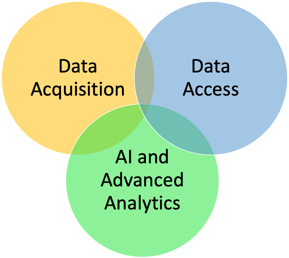
Fig. 6.1 Drivers of change in geospatial technology.#
Data Acquisition:
Earth Observation (EO) satellites were historically launched and operated by government agencies such as NASA, USGS, ESA, JAXA, ISRO, and others. While there were a few commercial companies starting to operate EO satellites in early 2000s, it was still very limited in scope. However, in the last decade with the advancements in smallsat and cubesat technologies a large number of commercial companies have entered the market and launched new satellite constellations. This boom in commercial EO satellites include launch of satellites that do not carry multi-spectral sensors, and instead carry synthetic aperture radar (SAR), light detection and ranging (Lidar), or Hyperspectral sensors.
Fig. 6.2 shows the growing archive of NASA satellite mission data as an example. and Fig. 6.3 shows collocated SAR and optical imagery.
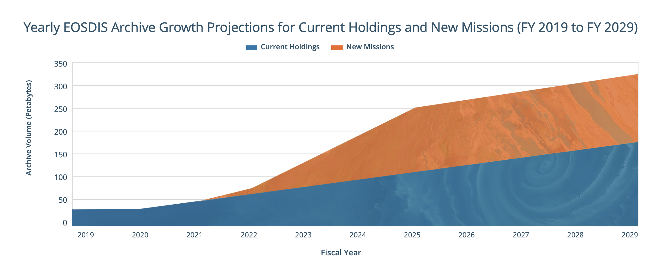
Fig. 6.2 Growing archive of NASA satellite mission data [source NASA Earth Data]#
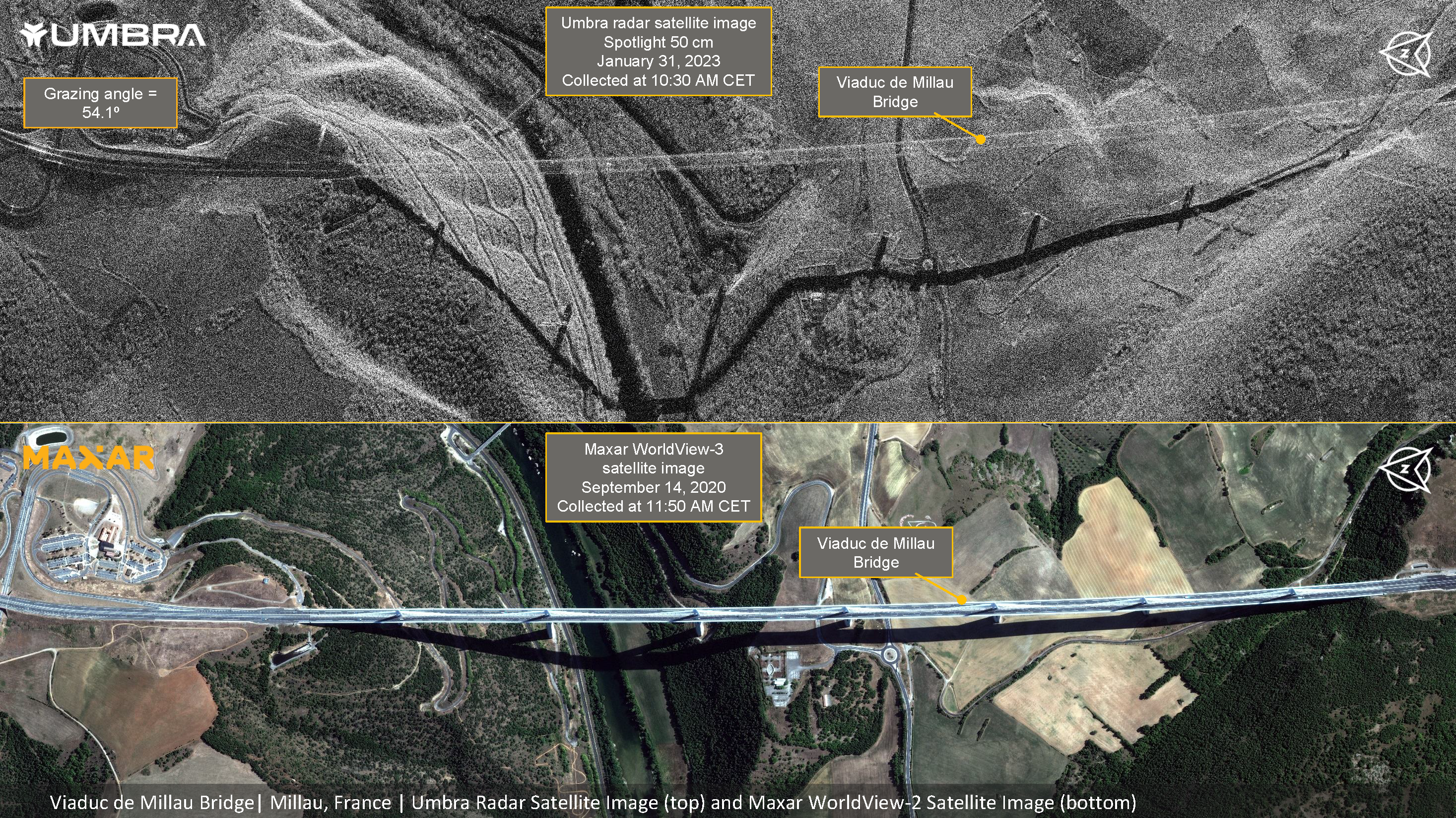
Fig. 6.3 Collocated SAR and optical imagery provided by Umbra and Maxar. [source: Umbra]#
Data Access
These new modes of data acquisition have resulted in new and innovate ways for storing, sharing and access these data. The traditional way of downloading all your imagery to your local machine (desktop or server) and running analysis on it does not scale anymore. It is more efficient, and in some case it’s the only possible solution, to bring the computation next to your data storage. The advancements in cloud technology has been a major help in changing how we access geospatial data these days.
The new mode of access also requires new data formats that are “cloud-native” and better ways of cataloging the data so users can query and find relevant data. (Read more about cloud-native geospatial data here).
Finally, these changes are accompanied by development of new APIs and data catalog standards that facilitate query and access of the data.
AI and Advanced Analytics
AI is revolutionizing how we consume data and what insights we can derive from data. Geospatial data is no exception in this case. There are numerous applications that are either enhanced by the use of AI or are purely enabled by them. Here is a non-inclusive list of such applications
Mapping non-forest trees in West Africa Sahara (link)
Mapping schools from space (link)
Mapping land use and land cover (link)
Mapping unmapped population (link)
Mapping Africa’s croplands (link)
These advancements require a new set of tools and pipeline for processing geospatial data, and hence have been one of the main drivers of changes in the geospatial Python landscape.
In the following sections, we will learn more about the geospatial technology landscape and in particular Python packages that facilitate usage and manipulation of geospatial data.
6.2. Cloud-native Data Formats#
Geospatial data is broadly categorized as vectors and rasters. With the changes that we talked about in the previous section, the file formats to store and access these data has evolved too. Let’s look at a similar example: back in the day you would buy/rent a DVD/CD or even cassette to watch a movie on your TV at home. Nowadays, you simply log into a website of app and “stream” the same type of content (with even higher image quality). Geospatial data is going through a similar change. You don’t want to download all the satellite images for your application, rather access them where they are stored and only load portions of the data needed for your analysis. Let’s deep dive into these concepts for each of raster and vector formats.
6.2.1. Raster Formats#
There are many formats for storing raster data. The most popular ones are:
GeoTIFF: This is a variant of TIFF (Tag Image File Format) format that is enriched with geospatial metadata. TIFF itself is the format mostly used by scanners and it has lossless compression schemes. In GeoTIFF files, the latitude and longitude at the edge of pixels is recorded in the header in addition to other metadata such as map projections, coordinate systems, datums, etc.
JPEG2000: This is a compress format for storing raster data that allows both lossy and lossless compressions.
netCDF: This is more that just a data format. According to UniData NetCDF page: NetCDF (network Common Data Form) is an interface for array-oriented data access and a library that provides an implementation of the interface. The netCDF library also defines a machine-independent format for representing scientific data. Together, the interface, library, and format support the creation, access, and sharing of scientific data. NetCDF is a widely used format for storing multi-dimensional geospatial data such as outputs of climate models.
Cloud Optimized GeoTIFF (COG): This is the cloud optimized version of GeoTIFF, and based on definition: is a regular GeoTIFF file, aimed at being hosted on a HTTP file server, with an internal organization that enables more efficient workflows on the cloud. It does this by leveraging the ability of clients issuing HTTP GET range requests to ask for just the parts of a file they need.
Cloud Optimized GeoTIFF relies on two complementary pieces of technology: The first is the ability of a GeoTIFF to not only store the raw pixels of the image, but to also organize those pixels in particular ways. The second is HTTP GET range requests, that let clients ask for just the portions of a file that they need. Together these enable fully online processing of data by COG-aware clients, as they can stream the right parts of the GeoTIFF as they need it, instead of having to download the whole file.
We will learn more about COGs in the next chapter.
Zarr: Zarr is a format for the storage of chunked, compressed, N-dimensional arrays inspired by HDF5, and NetCDF. From Zarr Spec: The primary motivation for the development of Zarr is to address this challenge by enabling the storage of large multidimensional arrays in a way that is compatible with parallel and/or distributed computing applications.
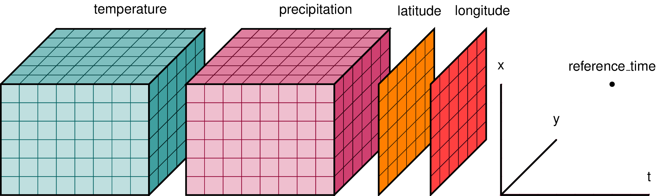
Fig. 6.4 Zarr data format used for storing n-dimensional arrays. An n-dimensional array is a great data model for dynamic phenomena. [source: Working with Climate Data]#
6.2.2. Vector Formats#
Similar to rasters, there are multiple formats for storing vector data. Here are a couple of the most popular ones:
Shapefile: are a popular geospatial vector data format. Shapefile was defined by ESRI and it’s supported by almost all geospatial software. Shapefile indeed refers to a collection files with the same filename but different extensions. Each shapefile contains four files: a .shp file, a .dbf file, a .shx file and a .prj file. These files store the the data itself, the location of the data, the index to share the data and the coordinate reference system. Such a way of storing the data make it hard to use on cloud object storages as the metadata about the data is stored in separate files and one has to access all of them to be able to query the dataset.
GeoJSON: GeoJSON is a format for encoding a variety of geographic data structures. From its spec: GeoJSON supports the following geometry types:
Point,LineString,Polygon,MultiPoint,MultiLineString, andMultiPolygon. Geometric objects with additional properties areFeatureobjects. Sets of features are contained byFeatureCollectionobjects.Check out this tutorial on creating and using GeoJSON.
GeoParquet: GeoParquet is a new evolving data format building on the powerful Apache Parquet format to add interoperable geospatial types (Point, Line and Polygon) to Parquet. You can read more about it here.
6.3. Open-Access Data#
Geospatial data has gone through major changes in terms of access policy in the last two decades. These changes which has mostly resulted in more open-access and free data has been a push for technology development.
Note: Open-access does not mean free by definition. Open-access refers to the license of the data which allows anyone to access it (sometimes this might be limited to certain usages like non-commercial). Open-access is an attribute of the data and does not mean the data is free or paid.
One of best examples of the free data policy, is Landsat data. Landsat satellite data was not free until 2008, and it was in that year that US Geological Survey (USGS) made Landsat data accessible for free. This resulted in substantial downloads of Landsat imagery and expansion of applications, and geospatial tools (check out this paper for more details). By some accounts, later in 2014 putting Landsat data on AWS cloud resulted in development of COG.
In recent years, there have been numerous developments to support publication and sharing of free datasets these include investments by government agencies in deploying data portals or providing grants to private institutions to do so, or by commercial companies who have allocated some of their resources to development and publication of open and free data.
6.4. SpatioTemporal Asset Catalog (STAC)#
The STAC specification is a common language to describe geospatial information, so it can more easily be worked with, indexed, and discovered. At its core, the SpatioTemporal Asset Catalog (STAC) specification provides a common structure for describing and cataloging spatiotemporal assets.
A spatiotemporal asset is any file that represents information about the earth captured in a certain space and time.
STAC is intentionally designed to be simple, flexible, and extensible. STAC is a network of JSON files that reference other JSON files, with each JSON file adhering to a specific core specification depending on which STAC component it is describing. This core JSON format can also be customized to fit differing needs, making the STAC specification highly flexible and adaptable. Check out this Intro to STAC guide to learn more about it.
In this course, we will interact with STAC data catalogs to search for geospatial data and retrieve them.
Another simple to use tool for STAC is STAC Browser. This browser retrieves a static catalog and you can browse it on the web.
6.5. Cloud Computing and Platforms#
6.6. Python Landscape#
Shapely
GDAL
Rasterio
GeoPandas
Xxarray and rioxarray
leafmap
Fiona
PyProj
Cartopy