7. Tutorial for Searching a STAC Catalog#
In this tutorial you will learn how to connect to a STAC API and search various datasets available for query. You will also search for specific items using a range of query parameters.
We will use the Earth Search API developed by Element84 for satellite datasets available on AWS S3 Storage (note that only those datasets that have a STAC catalog are served through this API). You can access the STAC catalog of the API here.
We will use the PySTAC pakcage for this tutorial. Check the documentation here, and these specific guides about using ItemSearch
You can find this notebook with a Dockerfile that contains all the required packages to run it on this repository.
Attribution: Parts of this notebook are inspired by the great tutorial on Access satellite imagery using Python (link)
from pystac_client import Client
api_url = "https://earth-search.aws.element84.com/v1"
client = Client.open(api_url)
7.1. Find Collections#
First, we would like to see what collections are available from this API.
collections = client.get_collections()
for collection in collections:
    print(collection)
<CollectionClient id=cop-dem-glo-30>
<CollectionClient id=naip>
<CollectionClient id=sentinel-2-l2a>
<CollectionClient id=sentinel-2-l1c>
<CollectionClient id=landsat-c2-l2>
<CollectionClient id=cop-dem-glo-90>
<CollectionClient id=sentinel-1-grd>
In order to get more information about a specific collection, you can use get_collection function:
s1_collection = client.get_collection("sentinel-1-grd")
s1_collection
- type "Collection"
- id "sentinel-1-grd"
- stac_version "1.0.0"
- description "Sentinel-1 is a pair of Synthetic Aperture Radar (SAR) imaging satellites launched in 2014 and 2016 by the European Space Agency (ESA). Their 6 day revisit cycle and ability to observe through clouds makes this dataset perfect for sea and land monitoring, emergency response due to environmental disasters, and economic applications. This dataset represents the global Sentinel-1 GRD archive, from beginning to the present, converted to cloud-optimized GeoTIFF format."
links [] 9 items
0
- rel "self"
- href "https://earth-search.aws.element84.com/v1/collections/sentinel-1-grd"
- type "application/json"
1
- rel "about"
- href "https://sentinels.copernicus.eu/web/sentinel/technical-guides/sentinel-1-sar/products-algorithms/level-1-algorithms/ground-range-detected"
- title "Sentinel-1 Ground Range Detected (GRD) Technical Guide"
2
- rel "license"
- href "https://sentinel.esa.int/documents/247904/690755/Sentinel_Data_Legal_Notice"
- title "Copernicus Sentinel data terms"
3
- rel "parent"
- href "https://earth-search.aws.element84.com/v1"
- type "application/json"
4
- rel "root"
- href "https://earth-search.aws.element84.com/v1"
- type "application/json"
- title "Earth Search by Element 84"
5
- rel "items"
- href "https://earth-search.aws.element84.com/v1/collections/sentinel-1-grd/items"
- type "application/geo+json"
6
- rel "http://www.opengis.net/def/rel/ogc/1.0/queryables"
- href "https://earth-search.aws.element84.com/v1/collections/sentinel-1-grd/queryables"
- type "application/schema+json"
7
- rel "aggregate"
- href "https://earth-search.aws.element84.com/v1/collections/sentinel-1-grd/aggregate"
- type "application/json"
- method "GET"
8
- rel "aggregations"
- href "https://earth-search.aws.element84.com/v1/collections/sentinel-1-grd/aggregations"
- type "application/json"
stac_extensions [] 5 items
- 0 "https://stac-extensions.github.io/storage/v1.0.0/schema.json"
- 1 "https://stac-extensions.github.io/sar/v1.0.0/schema.json"
- 2 "https://stac-extensions.github.io/sat/v1.0.0/schema.json"
- 3 "https://stac-extensions.github.io/item-assets/v1.0.0/schema.json"
- 4 "https://stac-extensions.github.io/raster/v1.1.0/schema.json"
item_assets
hh
- type "image/tiff; application=geotiff; profile=cloud-optimized"
roles [] 1 items
- 0 "data"
- title "HH Data"
raster:bands [] 1 items
0
- nodata 0
- data_type "uint16"
hv
- type "image/tiff; application=geotiff; profile=cloud-optimized"
roles [] 1 items
- 0 "data"
- title "HV Data"
raster:bands [] 1 items
0
- nodata 0
- data_type "uint16"
vh
- type "image/tiff; application=geotiff; profile=cloud-optimized"
roles [] 1 items
- 0 "data"
- title "VH Data"
raster:bands [] 1 items
0
- nodata 0
- data_type "uint16"
vv
- type "image/tiff; application=geotiff; profile=cloud-optimized"
roles [] 1 items
- 0 "data"
- title "VV Data"
raster:bands [] 1 items
0
- nodata 0
- data_type "uint16"
thumbnail
- type "image/png"
roles [] 1 items
- 0 "thumbnail"
- title "Thumbnail Image"
safe-manifest
- type "application/xml"
roles [] 1 items
- 0 "metadata"
- title "SAFE Manifest File"
schema-noise-hh
- type "application/xml"
roles [] 1 items
- 0 "metadata"
- title "HH Noise Schema"
schema-noise-hv
- type "application/xml"
roles [] 1 items
- 0 "metadata"
- title "HV Noise Schema"
schema-noise-vh
- type "application/xml"
roles [] 1 items
- 0 "metadata"
- title "VH Noise Schema"
schema-noise-vv
- type "application/xml"
roles [] 1 items
- 0 "metadata"
- title "VV Noise Schema"
schema-product-hh
- type "application/xml"
roles [] 1 items
- 0 "metadata"
- title "HH Product Schema"
schema-product-hv
- type "application/xml"
roles [] 1 items
- 0 "metadata"
- title "HV Product Schema"
schema-product-vh
- type "application/xml"
roles [] 1 items
- 0 "metadata"
- title "VH Product Schema"
schema-product-vv
- type "application/xml"
roles [] 1 items
- 0 "metadata"
- title "VV Product Schema"
schema-calibration-hh
- type "application/xml"
roles [] 1 items
- 0 "metadata"
- title "HH Calibration Schema"
schema-calibration-hv
- type "application/xml"
roles [] 1 items
- 0 "metadata"
- title "HV Calibration Schema"
schema-calibration-vh
- type "application/xml"
roles [] 1 items
- 0 "metadata"
- title "VH Calibration Schema"
schema-calibration-vv
- type "application/xml"
roles [] 1 items
- 0 "metadata"
- title "VV Calibration Schema"
- title "Sentinel-1 Level 1C Ground Range Detected (GRD)"
extent
spatial
bbox [] 1 items
0 [] 4 items
- 0 -180
- 1 -90
- 2 180
- 3 90
temporal
interval [] 1 items
0 [] 2 items
- 0 "2014-10-10T00:28:21Z"
- 1 None
- license "proprietary"
keywords [] 6 items
- 0 "ESA"
- 1 "Copernicus"
- 2 "Sentinel"
- 3 "C-Band"
- 4 "SAR"
- 5 "GRD"
providers [] 3 items
0
- name "ESA"
roles [] 3 items
- 0 "producer"
- 1 "processor"
- 2 "licensor"
- url "https://earth.esa.int/web/guest/home"
1
- name "AWS"
roles [] 1 items
- 0 "host"
- url "https://registry.opendata.aws/sentinel-1"
2
- name "Element 84"
roles [] 1 items
- 0 "processor"
- url "https://element84.com"
summaries
platform [] 2 items
- 0 "sentinel-1a"
- 1 "sentinel-1b"
constellation [] 1 items
- 0 "sentinel-1"
s1:resolution [] 3 items
- 0 "full"
- 1 "high"
- 2 "medium"
s1:orbit_source [] 4 items
- 0 "DOWNLINK"
- 1 "POEORB"
- 2 "PREORB"
- 3 "RESORB"
sar:looks_range [] 4 items
- 0 5
- 1 6
- 2 3
- 3 2
sat:orbit_state [] 2 items
- 0 "ascending"
- 1 "descending"
sar:product_type [] 1 items
- 0 "GRD"
sar:looks_azimuth [] 3 items
- 0 1
- 1 6
- 2 2
sar:polarizations [] 6 items
0 [] 2 items
- 0 "VV"
- 1 "VH"
1 [] 2 items
- 0 "HH"
- 1 "HV"
2 [] 1 items
- 0 "VV"
3 [] 1 items
- 0 "VH"
4 [] 1 items
- 0 "HH"
5 [] 1 items
- 0 "HV"
sar:frequency_band [] 1 items
- 0 "C"
s1:processing_level [] 1 items
- 0 "1"
sar:instrument_mode [] 3 items
- 0 "IW"
- 1 "EW"
- 2 "SM"
sar:center_frequency [] 1 items
- 0 5.405
sar:resolution_range [] 5 items
- 0 20
- 1 23
- 2 50
- 3 93
- 4 9
s1:product_timeliness [] 6 items
- 0 "NRT-10m"
- 1 "NRT-1h"
- 2 "NRT-3h"
- 3 "Fast-24h"
- 4 "Off-line"
- 5 "Reprocessing"
sar:resolution_azimuth [] 5 items
- 0 22
- 1 23
- 2 50
- 3 87
- 4 9
sar:pixel_spacing_range [] 4 items
- 0 10
- 1 25
- 2 40
- 3 3.5
sar:observation_direction [] 1 items
- 0 "right"
sar:pixel_spacing_azimuth [] 4 items
- 0 10
- 1 25
- 2 40
- 3 3.5
sar:looks_equivalent_number [] 5 items
- 0 4.4
- 1 29.7
- 2 2.7
- 3 10.7
- 4 3.7
sat:platform_international_designator [] 3 items
- 0 "2014-016A"
- 1 "2016-025A"
- 2 "0000-000A"
storage:platform [] 1 items
- 0 "AWS"
storage:region [] 1 items
- 0 "eu-central-1"
storage:requester_pays [] 1 items
- 0 True
7.2. Search Items#
Let’s use Leafmap to select a point where we are interested to find a satellite imagery
import leafmap
m = leafmap.Map(center=[42.250809, -71.822833], zoom=16, height="800px")
m
Pan and zoom the map to find an area of interest, then use the tools on the top left of the map to select a point on the map.
if m.user_rois is not None:
    point = m.user_rois['features'][0]['geometry']
else:
    point = dict(type="Point", coordinates=(42.250809, -71.822833))
We are interested to search for Sentinel-2 imagery that intersects with the point we selected in the previous step. So we will use the search function and insert sentinel-2-l2a as our collection of interest. We also use the intersects property to filter the scenes that intersect with our point of interest.
search_results = client.search(
    collections=["sentinel-2-l2a"],
    intersects=point,
    max_items=12,
)
print(search_results.matched())
1928
The number that is returned in the previous step is more than 12 that we had identified in our search criteria. But this doesn’t mean all the metadata about these scenes haven been retrieved. This just shows how many scenes have matched our search criteria. In the next cell, we will call item_collection() to retrieve the metadata, and check how many of them are retrieved.
items = search_results.item_collection()
len(items)
12
Now, let’s investigate an item
items[0]
- type "Feature"
- stac_version "1.0.0"
- id "S2A_18TYM_20230926_0_L2A"
properties
- created "2023-09-26T23:03:26.333Z"
- platform "sentinel-2a"
- constellation "sentinel-2"
instruments [] 1 items
- 0 "msi"
- eo:cloud_cover 98.445553
- proj:epsg 32618
- mgrs:utm_zone 18
- mgrs:latitude_band "T"
- mgrs:grid_square "YM"
- grid:code "MGRS-18TYM"
- view:sun_azimuth 159.514180885773
- view:sun_elevation 44.854597440896
- s2:degraded_msi_data_percentage 0.0244
- s2:nodata_pixel_percentage 48.157543
- s2:saturated_defective_pixel_percentage 0
- s2:dark_features_percentage 0
- s2:cloud_shadow_percentage 1.465521
- s2:vegetation_percentage 0
- s2:not_vegetated_percentage 6e-06
- s2:water_percentage 0.088555
- s2:unclassified_percentage 0.000365
- s2:medium_proba_clouds_percentage 26.676089
- s2:high_proba_clouds_percentage 67.755795
- s2:thin_cirrus_percentage 4.013672
- s2:snow_ice_percentage 0
- s2:product_type "S2MSI2A"
- s2:processing_baseline "05.09"
- s2:product_uri "S2A_MSIL2A_20230926T153601_N0509_R111_T18TYM_20230926T204656.SAFE"
- s2:generation_time "2023-09-26T20:46:56.000000Z"
- s2:datatake_id "GS2A_20230926T153601_043151_N05.09"
- s2:datatake_type "INS-NOBS"
- s2:datastrip_id "S2A_OPER_MSI_L2A_DS_2APS_20230926T204656_S20230926T153557_N05.09"
- s2:granule_id "S2A_OPER_MSI_L2A_TL_2APS_20230926T204656_A043151_T18TYM_N05.09"
- s2:reflectance_conversion_factor 0.993270756881969
- datetime "2023-09-26T15:41:35.094000Z"
- s2:sequence "0"
- earthsearch:s3_path "s3://sentinel-cogs/sentinel-s2-l2a-cogs/18/T/YM/2023/9/S2A_18TYM_20230926_0_L2A"
- earthsearch:payload_id "roda-sentinel2/workflow-sentinel2-to-stac/bea3e963d459033018883bfc5e1c42cc"
- earthsearch:boa_offset_applied True
processing:software
- sentinel2-to-stac "0.1.1"
- updated "2023-09-26T23:03:26.333Z"
geometry
- type "Polygon"
coordinates [] 1 items
0 [] 5 items
0 [] 2 items
- 0 -71.79498386317441
- 1 42.40785435022417
1 [] 2 items
- 0 -72.10290249964824
- 1 41.427267029114304
2 [] 2 items
- 0 -71.2944491287618
- 1 41.4040441194201
3 [] 2 items
- 0 -71.23687622798481
- 1 42.390872073839105
4 [] 2 items
- 0 -71.79498386317441
- 1 42.40785435022417
links [] 8 items
0
- rel "self"
- href "https://earth-search.aws.element84.com/v1/collections/sentinel-2-l2a/items/S2A_18TYM_20230926_0_L2A"
- type "application/geo+json"
1
- rel "canonical"
- href "s3://sentinel-cogs/sentinel-s2-l2a-cogs/18/T/YM/2023/9/S2A_18TYM_20230926_0_L2A/S2A_18TYM_20230926_0_L2A.json"
- type "application/json"
2
- rel "license"
- href "https://sentinel.esa.int/documents/247904/690755/Sentinel_Data_Legal_Notice"
3
- rel "derived_from"
- href "https://earth-search.aws.element84.com/v1/collections/sentinel-2-l1c/items/S2A_18TYM_20230926_0_L1C"
- type "application/geo+json"
4
- rel "parent"
- href "https://earth-search.aws.element84.com/v1/collections/sentinel-2-l2a"
- type "application/json"
5
- rel "collection"
- href "https://earth-search.aws.element84.com/v1/collections/sentinel-2-l2a"
- type "application/json"
6
- rel "root"
- href "https://earth-search.aws.element84.com/v1"
- type "application/json"
- title "Earth Search by Element 84"
7
- rel "thumbnail"
- href "https://earth-search.aws.element84.com/v1/collections/sentinel-2-l2a/items/S2A_18TYM_20230926_0_L2A/thumbnail"
assets
aot
- href "https://sentinel-cogs.s3.us-west-2.amazonaws.com/sentinel-s2-l2a-cogs/18/T/YM/2023/9/S2A_18TYM_20230926_0_L2A/AOT.tif"
- type "image/tiff; application=geotiff; profile=cloud-optimized"
- title "Aerosol optical thickness (AOT)"
proj:shape [] 2 items
- 0 5490
- 1 5490
proj:transform [] 6 items
- 0 20
- 1 0
- 2 699960
- 3 0
- 4 -20
- 5 4700040
raster:bands [] 1 items
0
- nodata 0
- data_type "uint16"
- bits_per_sample 15
- spatial_resolution 20
- scale 0.001
- offset 0
roles [] 2 items
- 0 "data"
- 1 "reflectance"
blue
- href "https://sentinel-cogs.s3.us-west-2.amazonaws.com/sentinel-s2-l2a-cogs/18/T/YM/2023/9/S2A_18TYM_20230926_0_L2A/B02.tif"
- type "image/tiff; application=geotiff; profile=cloud-optimized"
- title "Blue (band 2) - 10m"
eo:bands [] 1 items
0
- name "blue"
- common_name "blue"
- description "Blue (band 2)"
- center_wavelength 0.49
- full_width_half_max 0.098
- gsd 10
proj:shape [] 2 items
- 0 10980
- 1 10980
proj:transform [] 6 items
- 0 10
- 1 0
- 2 699960
- 3 0
- 4 -10
- 5 4700040
raster:bands [] 1 items
0
- nodata 0
- data_type "uint16"
- bits_per_sample 15
- spatial_resolution 10
- scale 0.0001
- offset -0.1
roles [] 2 items
- 0 "data"
- 1 "reflectance"
coastal
- href "https://sentinel-cogs.s3.us-west-2.amazonaws.com/sentinel-s2-l2a-cogs/18/T/YM/2023/9/S2A_18TYM_20230926_0_L2A/B01.tif"
- type "image/tiff; application=geotiff; profile=cloud-optimized"
- title "Coastal aerosol (band 1) - 60m"
eo:bands [] 1 items
0
- name "coastal"
- common_name "coastal"
- description "Coastal aerosol (band 1)"
- center_wavelength 0.443
- full_width_half_max 0.027
- gsd 60
proj:shape [] 2 items
- 0 1830
- 1 1830
proj:transform [] 6 items
- 0 60
- 1 0
- 2 699960
- 3 0
- 4 -60
- 5 4700040
raster:bands [] 1 items
0
- nodata 0
- data_type "uint16"
- bits_per_sample 15
- spatial_resolution 60
- scale 0.0001
- offset -0.1
roles [] 2 items
- 0 "data"
- 1 "reflectance"
granule_metadata
- href "https://sentinel-cogs.s3.us-west-2.amazonaws.com/sentinel-s2-l2a-cogs/18/T/YM/2023/9/S2A_18TYM_20230926_0_L2A/granule_metadata.xml"
- type "application/xml"
roles [] 1 items
- 0 "metadata"
green
- href "https://sentinel-cogs.s3.us-west-2.amazonaws.com/sentinel-s2-l2a-cogs/18/T/YM/2023/9/S2A_18TYM_20230926_0_L2A/B03.tif"
- type "image/tiff; application=geotiff; profile=cloud-optimized"
- title "Green (band 3) - 10m"
eo:bands [] 1 items
0
- name "green"
- common_name "green"
- description "Green (band 3)"
- center_wavelength 0.56
- full_width_half_max 0.045
- gsd 10
proj:shape [] 2 items
- 0 10980
- 1 10980
proj:transform [] 6 items
- 0 10
- 1 0
- 2 699960
- 3 0
- 4 -10
- 5 4700040
raster:bands [] 1 items
0
- nodata 0
- data_type "uint16"
- bits_per_sample 15
- spatial_resolution 10
- scale 0.0001
- offset -0.1
roles [] 2 items
- 0 "data"
- 1 "reflectance"
nir
- href "https://sentinel-cogs.s3.us-west-2.amazonaws.com/sentinel-s2-l2a-cogs/18/T/YM/2023/9/S2A_18TYM_20230926_0_L2A/B08.tif"
- type "image/tiff; application=geotiff; profile=cloud-optimized"
- title "NIR 1 (band 8) - 10m"
eo:bands [] 1 items
0
- name "nir"
- common_name "nir"
- description "NIR 1 (band 8)"
- center_wavelength 0.842
- full_width_half_max 0.145
- gsd 10
proj:shape [] 2 items
- 0 10980
- 1 10980
proj:transform [] 6 items
- 0 10
- 1 0
- 2 699960
- 3 0
- 4 -10
- 5 4700040
raster:bands [] 1 items
0
- nodata 0
- data_type "uint16"
- bits_per_sample 15
- spatial_resolution 10
- scale 0.0001
- offset -0.1
roles [] 2 items
- 0 "data"
- 1 "reflectance"
nir08
- href "https://sentinel-cogs.s3.us-west-2.amazonaws.com/sentinel-s2-l2a-cogs/18/T/YM/2023/9/S2A_18TYM_20230926_0_L2A/B8A.tif"
- type "image/tiff; application=geotiff; profile=cloud-optimized"
- title "NIR 2 (band 8A) - 20m"
eo:bands [] 1 items
0
- name "nir08"
- common_name "nir08"
- description "NIR 2 (band 8A)"
- center_wavelength 0.865
- full_width_half_max 0.033
- gsd 20
proj:shape [] 2 items
- 0 5490
- 1 5490
proj:transform [] 6 items
- 0 20
- 1 0
- 2 699960
- 3 0
- 4 -20
- 5 4700040
raster:bands [] 1 items
0
- nodata 0
- data_type "uint16"
- bits_per_sample 15
- spatial_resolution 20
- scale 0.0001
- offset -0.1
roles [] 2 items
- 0 "data"
- 1 "reflectance"
nir09
- href "https://sentinel-cogs.s3.us-west-2.amazonaws.com/sentinel-s2-l2a-cogs/18/T/YM/2023/9/S2A_18TYM_20230926_0_L2A/B09.tif"
- type "image/tiff; application=geotiff; profile=cloud-optimized"
- title "NIR 3 (band 9) - 60m"
eo:bands [] 1 items
0
- name "nir09"
- common_name "nir09"
- description "NIR 3 (band 9)"
- center_wavelength 0.945
- full_width_half_max 0.026
- gsd 60
proj:shape [] 2 items
- 0 1830
- 1 1830
proj:transform [] 6 items
- 0 60
- 1 0
- 2 699960
- 3 0
- 4 -60
- 5 4700040
raster:bands [] 1 items
0
- nodata 0
- data_type "uint16"
- bits_per_sample 15
- spatial_resolution 60
- scale 0.0001
- offset -0.1
roles [] 2 items
- 0 "data"
- 1 "reflectance"
red
- href "https://sentinel-cogs.s3.us-west-2.amazonaws.com/sentinel-s2-l2a-cogs/18/T/YM/2023/9/S2A_18TYM_20230926_0_L2A/B04.tif"
- type "image/tiff; application=geotiff; profile=cloud-optimized"
- title "Red (band 4) - 10m"
eo:bands [] 1 items
0
- name "red"
- common_name "red"
- description "Red (band 4)"
- center_wavelength 0.665
- full_width_half_max 0.038
- gsd 10
proj:shape [] 2 items
- 0 10980
- 1 10980
proj:transform [] 6 items
- 0 10
- 1 0
- 2 699960
- 3 0
- 4 -10
- 5 4700040
raster:bands [] 1 items
0
- nodata 0
- data_type "uint16"
- bits_per_sample 15
- spatial_resolution 10
- scale 0.0001
- offset -0.1
roles [] 2 items
- 0 "data"
- 1 "reflectance"
rededge1
- href "https://sentinel-cogs.s3.us-west-2.amazonaws.com/sentinel-s2-l2a-cogs/18/T/YM/2023/9/S2A_18TYM_20230926_0_L2A/B05.tif"
- type "image/tiff; application=geotiff; profile=cloud-optimized"
- title "Red edge 1 (band 5) - 20m"
eo:bands [] 1 items
0
- name "rededge1"
- common_name "rededge"
- description "Red edge 1 (band 5)"
- center_wavelength 0.704
- full_width_half_max 0.019
- gsd 20
proj:shape [] 2 items
- 0 5490
- 1 5490
proj:transform [] 6 items
- 0 20
- 1 0
- 2 699960
- 3 0
- 4 -20
- 5 4700040
raster:bands [] 1 items
0
- nodata 0
- data_type "uint16"
- bits_per_sample 15
- spatial_resolution 20
- scale 0.0001
- offset -0.1
roles [] 2 items
- 0 "data"
- 1 "reflectance"
rededge2
- href "https://sentinel-cogs.s3.us-west-2.amazonaws.com/sentinel-s2-l2a-cogs/18/T/YM/2023/9/S2A_18TYM_20230926_0_L2A/B06.tif"
- type "image/tiff; application=geotiff; profile=cloud-optimized"
- title "Red edge 2 (band 6) - 20m"
eo:bands [] 1 items
0
- name "rededge2"
- common_name "rededge"
- description "Red edge 2 (band 6)"
- center_wavelength 0.74
- full_width_half_max 0.018
- gsd 20
proj:shape [] 2 items
- 0 5490
- 1 5490
proj:transform [] 6 items
- 0 20
- 1 0
- 2 699960
- 3 0
- 4 -20
- 5 4700040
raster:bands [] 1 items
0
- nodata 0
- data_type "uint16"
- bits_per_sample 15
- spatial_resolution 20
- scale 0.0001
- offset -0.1
roles [] 2 items
- 0 "data"
- 1 "reflectance"
rededge3
- href "https://sentinel-cogs.s3.us-west-2.amazonaws.com/sentinel-s2-l2a-cogs/18/T/YM/2023/9/S2A_18TYM_20230926_0_L2A/B07.tif"
- type "image/tiff; application=geotiff; profile=cloud-optimized"
- title "Red edge 3 (band 7) - 20m"
eo:bands [] 1 items
0
- name "rededge3"
- common_name "rededge"
- description "Red edge 3 (band 7)"
- center_wavelength 0.783
- full_width_half_max 0.028
- gsd 20
proj:shape [] 2 items
- 0 5490
- 1 5490
proj:transform [] 6 items
- 0 20
- 1 0
- 2 699960
- 3 0
- 4 -20
- 5 4700040
raster:bands [] 1 items
0
- nodata 0
- data_type "uint16"
- bits_per_sample 15
- spatial_resolution 20
- scale 0.0001
- offset -0.1
roles [] 2 items
- 0 "data"
- 1 "reflectance"
scl
- href "https://sentinel-cogs.s3.us-west-2.amazonaws.com/sentinel-s2-l2a-cogs/18/T/YM/2023/9/S2A_18TYM_20230926_0_L2A/SCL.tif"
- type "image/tiff; application=geotiff; profile=cloud-optimized"
- title "Scene classification map (SCL)"
proj:shape [] 2 items
- 0 5490
- 1 5490
proj:transform [] 6 items
- 0 20
- 1 0
- 2 699960
- 3 0
- 4 -20
- 5 4700040
raster:bands [] 1 items
0
- nodata 0
- data_type "uint8"
- spatial_resolution 20
roles [] 2 items
- 0 "data"
- 1 "reflectance"
swir16
- href "https://sentinel-cogs.s3.us-west-2.amazonaws.com/sentinel-s2-l2a-cogs/18/T/YM/2023/9/S2A_18TYM_20230926_0_L2A/B11.tif"
- type "image/tiff; application=geotiff; profile=cloud-optimized"
- title "SWIR 1 (band 11) - 20m"
eo:bands [] 1 items
0
- name "swir16"
- common_name "swir16"
- description "SWIR 1 (band 11)"
- center_wavelength 1.61
- full_width_half_max 0.143
- gsd 20
proj:shape [] 2 items
- 0 5490
- 1 5490
proj:transform [] 6 items
- 0 20
- 1 0
- 2 699960
- 3 0
- 4 -20
- 5 4700040
raster:bands [] 1 items
0
- nodata 0
- data_type "uint16"
- bits_per_sample 15
- spatial_resolution 20
- scale 0.0001
- offset -0.1
roles [] 2 items
- 0 "data"
- 1 "reflectance"
swir22
- href "https://sentinel-cogs.s3.us-west-2.amazonaws.com/sentinel-s2-l2a-cogs/18/T/YM/2023/9/S2A_18TYM_20230926_0_L2A/B12.tif"
- type "image/tiff; application=geotiff; profile=cloud-optimized"
- title "SWIR 2 (band 12) - 20m"
eo:bands [] 1 items
0
- name "swir22"
- common_name "swir22"
- description "SWIR 2 (band 12)"
- center_wavelength 2.19
- full_width_half_max 0.242
- gsd 20
proj:shape [] 2 items
- 0 5490
- 1 5490
proj:transform [] 6 items
- 0 20
- 1 0
- 2 699960
- 3 0
- 4 -20
- 5 4700040
raster:bands [] 1 items
0
- nodata 0
- data_type "uint16"
- bits_per_sample 15
- spatial_resolution 20
- scale 0.0001
- offset -0.1
roles [] 2 items
- 0 "data"
- 1 "reflectance"
thumbnail
- href "https://sentinel-cogs.s3.us-west-2.amazonaws.com/sentinel-s2-l2a-cogs/18/T/YM/2023/9/S2A_18TYM_20230926_0_L2A/thumbnail.jpg"
- type "image/jpeg"
- title "Thumbnail image"
roles [] 1 items
- 0 "thumbnail"
tileinfo_metadata
- href "https://sentinel-cogs.s3.us-west-2.amazonaws.com/sentinel-s2-l2a-cogs/18/T/YM/2023/9/S2A_18TYM_20230926_0_L2A/tileinfo_metadata.json"
- type "application/json"
roles [] 1 items
- 0 "metadata"
visual
- href "https://sentinel-cogs.s3.us-west-2.amazonaws.com/sentinel-s2-l2a-cogs/18/T/YM/2023/9/S2A_18TYM_20230926_0_L2A/TCI.tif"
- type "image/tiff; application=geotiff; profile=cloud-optimized"
- title "True color image"
eo:bands [] 3 items
0
- name "red"
- common_name "red"
- description "Red (band 4)"
- center_wavelength 0.665
- full_width_half_max 0.038
1
- name "green"
- common_name "green"
- description "Green (band 3)"
- center_wavelength 0.56
- full_width_half_max 0.045
2
- name "blue"
- common_name "blue"
- description "Blue (band 2)"
- center_wavelength 0.49
- full_width_half_max 0.098
proj:shape [] 2 items
- 0 10980
- 1 10980
proj:transform [] 6 items
- 0 10
- 1 0
- 2 699960
- 3 0
- 4 -10
- 5 4700040
roles [] 1 items
- 0 "visual"
wvp
- href "https://sentinel-cogs.s3.us-west-2.amazonaws.com/sentinel-s2-l2a-cogs/18/T/YM/2023/9/S2A_18TYM_20230926_0_L2A/WVP.tif"
- type "image/tiff; application=geotiff; profile=cloud-optimized"
- title "Water vapour (WVP)"
proj:shape [] 2 items
- 0 5490
- 1 5490
proj:transform [] 6 items
- 0 20
- 1 0
- 2 699960
- 3 0
- 4 -20
- 5 4700040
raster:bands [] 1 items
0
- nodata 0
- data_type "uint16"
- bits_per_sample 15
- spatial_resolution 20
- unit "cm"
- scale 0.001
- offset 0
roles [] 2 items
- 0 "data"
- 1 "reflectance"
aot-jp2
- href "s3://sentinel-s2-l2a/tiles/18/T/YM/2023/9/26/0/AOT.jp2"
- type "image/jp2"
- title "Aerosol optical thickness (AOT)"
proj:shape [] 2 items
- 0 5490
- 1 5490
proj:transform [] 6 items
- 0 20
- 1 0
- 2 699960
- 3 0
- 4 -20
- 5 4700040
raster:bands [] 1 items
0
- nodata 0
- data_type "uint16"
- bits_per_sample 15
- spatial_resolution 20
- scale 0.001
- offset 0
roles [] 2 items
- 0 "data"
- 1 "reflectance"
blue-jp2
- href "s3://sentinel-s2-l2a/tiles/18/T/YM/2023/9/26/0/B02.jp2"
- type "image/jp2"
- title "Blue (band 2) - 10m"
eo:bands [] 1 items
0
- name "blue"
- common_name "blue"
- description "Blue (band 2)"
- center_wavelength 0.49
- full_width_half_max 0.098
- gsd 10
proj:shape [] 2 items
- 0 10980
- 1 10980
proj:transform [] 6 items
- 0 10
- 1 0
- 2 699960
- 3 0
- 4 -10
- 5 4700040
raster:bands [] 1 items
0
- nodata 0
- data_type "uint16"
- bits_per_sample 15
- spatial_resolution 10
- scale 0.0001
- offset -0.1
roles [] 2 items
- 0 "data"
- 1 "reflectance"
coastal-jp2
- href "s3://sentinel-s2-l2a/tiles/18/T/YM/2023/9/26/0/B01.jp2"
- type "image/jp2"
- title "Coastal aerosol (band 1) - 60m"
eo:bands [] 1 items
0
- name "coastal"
- common_name "coastal"
- description "Coastal aerosol (band 1)"
- center_wavelength 0.443
- full_width_half_max 0.027
- gsd 60
proj:shape [] 2 items
- 0 1830
- 1 1830
proj:transform [] 6 items
- 0 60
- 1 0
- 2 699960
- 3 0
- 4 -60
- 5 4700040
raster:bands [] 1 items
0
- nodata 0
- data_type "uint16"
- bits_per_sample 15
- spatial_resolution 60
- scale 0.0001
- offset -0.1
roles [] 2 items
- 0 "data"
- 1 "reflectance"
green-jp2
- href "s3://sentinel-s2-l2a/tiles/18/T/YM/2023/9/26/0/B03.jp2"
- type "image/jp2"
- title "Green (band 3) - 10m"
eo:bands [] 1 items
0
- name "green"
- common_name "green"
- description "Green (band 3)"
- center_wavelength 0.56
- full_width_half_max 0.045
- gsd 10
proj:shape [] 2 items
- 0 10980
- 1 10980
proj:transform [] 6 items
- 0 10
- 1 0
- 2 699960
- 3 0
- 4 -10
- 5 4700040
raster:bands [] 1 items
0
- nodata 0
- data_type "uint16"
- bits_per_sample 15
- spatial_resolution 10
- scale 0.0001
- offset -0.1
roles [] 2 items
- 0 "data"
- 1 "reflectance"
nir-jp2
- href "s3://sentinel-s2-l2a/tiles/18/T/YM/2023/9/26/0/B08.jp2"
- type "image/jp2"
- title "NIR 1 (band 8) - 10m"
eo:bands [] 1 items
0
- name "nir"
- common_name "nir"
- description "NIR 1 (band 8)"
- center_wavelength 0.842
- full_width_half_max 0.145
- gsd 10
proj:shape [] 2 items
- 0 10980
- 1 10980
proj:transform [] 6 items
- 0 10
- 1 0
- 2 699960
- 3 0
- 4 -10
- 5 4700040
raster:bands [] 1 items
0
- nodata 0
- data_type "uint16"
- bits_per_sample 15
- spatial_resolution 10
- scale 0.0001
- offset -0.1
roles [] 2 items
- 0 "data"
- 1 "reflectance"
nir08-jp2
- href "s3://sentinel-s2-l2a/tiles/18/T/YM/2023/9/26/0/B8A.jp2"
- type "image/jp2"
- title "NIR 2 (band 8A) - 20m"
eo:bands [] 1 items
0
- name "nir08"
- common_name "nir08"
- description "NIR 2 (band 8A)"
- center_wavelength 0.865
- full_width_half_max 0.033
- gsd 20
proj:shape [] 2 items
- 0 5490
- 1 5490
proj:transform [] 6 items
- 0 20
- 1 0
- 2 699960
- 3 0
- 4 -20
- 5 4700040
raster:bands [] 1 items
0
- nodata 0
- data_type "uint16"
- bits_per_sample 15
- spatial_resolution 20
- scale 0.0001
- offset -0.1
roles [] 2 items
- 0 "data"
- 1 "reflectance"
nir09-jp2
- href "s3://sentinel-s2-l2a/tiles/18/T/YM/2023/9/26/0/B09.jp2"
- type "image/jp2"
- title "NIR 3 (band 9) - 60m"
eo:bands [] 1 items
0
- name "nir09"
- common_name "nir09"
- description "NIR 3 (band 9)"
- center_wavelength 0.945
- full_width_half_max 0.026
- gsd 60
proj:shape [] 2 items
- 0 1830
- 1 1830
proj:transform [] 6 items
- 0 60
- 1 0
- 2 699960
- 3 0
- 4 -60
- 5 4700040
raster:bands [] 1 items
0
- nodata 0
- data_type "uint16"
- bits_per_sample 15
- spatial_resolution 60
- scale 0.0001
- offset -0.1
roles [] 2 items
- 0 "data"
- 1 "reflectance"
red-jp2
- href "s3://sentinel-s2-l2a/tiles/18/T/YM/2023/9/26/0/B04.jp2"
- type "image/jp2"
- title "Red (band 4) - 10m"
eo:bands [] 1 items
0
- name "red"
- common_name "red"
- description "Red (band 4)"
- center_wavelength 0.665
- full_width_half_max 0.038
- gsd 10
proj:shape [] 2 items
- 0 10980
- 1 10980
proj:transform [] 6 items
- 0 10
- 1 0
- 2 699960
- 3 0
- 4 -10
- 5 4700040
raster:bands [] 1 items
0
- nodata 0
- data_type "uint16"
- bits_per_sample 15
- spatial_resolution 10
- scale 0.0001
- offset -0.1
roles [] 2 items
- 0 "data"
- 1 "reflectance"
rededge1-jp2
- href "s3://sentinel-s2-l2a/tiles/18/T/YM/2023/9/26/0/B05.jp2"
- type "image/jp2"
- title "Red edge 1 (band 5) - 20m"
eo:bands [] 1 items
0
- name "rededge1"
- common_name "rededge"
- description "Red edge 1 (band 5)"
- center_wavelength 0.704
- full_width_half_max 0.019
- gsd 20
proj:shape [] 2 items
- 0 5490
- 1 5490
proj:transform [] 6 items
- 0 20
- 1 0
- 2 699960
- 3 0
- 4 -20
- 5 4700040
raster:bands [] 1 items
0
- nodata 0
- data_type "uint16"
- bits_per_sample 15
- spatial_resolution 20
- scale 0.0001
- offset -0.1
roles [] 2 items
- 0 "data"
- 1 "reflectance"
rededge2-jp2
- href "s3://sentinel-s2-l2a/tiles/18/T/YM/2023/9/26/0/B06.jp2"
- type "image/jp2"
- title "Red edge 2 (band 6) - 20m"
eo:bands [] 1 items
0
- name "rededge2"
- common_name "rededge"
- description "Red edge 2 (band 6)"
- center_wavelength 0.74
- full_width_half_max 0.018
- gsd 20
proj:shape [] 2 items
- 0 5490
- 1 5490
proj:transform [] 6 items
- 0 20
- 1 0
- 2 699960
- 3 0
- 4 -20
- 5 4700040
raster:bands [] 1 items
0
- nodata 0
- data_type "uint16"
- bits_per_sample 15
- spatial_resolution 20
- scale 0.0001
- offset -0.1
roles [] 2 items
- 0 "data"
- 1 "reflectance"
rededge3-jp2
- href "s3://sentinel-s2-l2a/tiles/18/T/YM/2023/9/26/0/B07.jp2"
- type "image/jp2"
- title "Red edge 3 (band 7) - 20m"
eo:bands [] 1 items
0
- name "rededge3"
- common_name "rededge"
- description "Red edge 3 (band 7)"
- center_wavelength 0.783
- full_width_half_max 0.028
- gsd 20
proj:shape [] 2 items
- 0 5490
- 1 5490
proj:transform [] 6 items
- 0 20
- 1 0
- 2 699960
- 3 0
- 4 -20
- 5 4700040
raster:bands [] 1 items
0
- nodata 0
- data_type "uint16"
- bits_per_sample 15
- spatial_resolution 20
- scale 0.0001
- offset -0.1
roles [] 2 items
- 0 "data"
- 1 "reflectance"
scl-jp2
- href "s3://sentinel-s2-l2a/tiles/18/T/YM/2023/9/26/0/SCL.jp2"
- type "image/jp2"
- title "Scene classification map (SCL)"
proj:shape [] 2 items
- 0 5490
- 1 5490
proj:transform [] 6 items
- 0 20
- 1 0
- 2 699960
- 3 0
- 4 -20
- 5 4700040
raster:bands [] 1 items
0
- nodata 0
- data_type "uint8"
- spatial_resolution 20
roles [] 2 items
- 0 "data"
- 1 "reflectance"
swir16-jp2
- href "s3://sentinel-s2-l2a/tiles/18/T/YM/2023/9/26/0/B11.jp2"
- type "image/jp2"
- title "SWIR 1 (band 11) - 20m"
eo:bands [] 1 items
0
- name "swir16"
- common_name "swir16"
- description "SWIR 1 (band 11)"
- center_wavelength 1.61
- full_width_half_max 0.143
- gsd 20
proj:shape [] 2 items
- 0 5490
- 1 5490
proj:transform [] 6 items
- 0 20
- 1 0
- 2 699960
- 3 0
- 4 -20
- 5 4700040
raster:bands [] 1 items
0
- nodata 0
- data_type "uint16"
- bits_per_sample 15
- spatial_resolution 20
- scale 0.0001
- offset -0.1
roles [] 2 items
- 0 "data"
- 1 "reflectance"
swir22-jp2
- href "s3://sentinel-s2-l2a/tiles/18/T/YM/2023/9/26/0/B12.jp2"
- type "image/jp2"
- title "SWIR 2 (band 12) - 20m"
eo:bands [] 1 items
0
- name "swir22"
- common_name "swir22"
- description "SWIR 2 (band 12)"
- center_wavelength 2.19
- full_width_half_max 0.242
- gsd 20
proj:shape [] 2 items
- 0 5490
- 1 5490
proj:transform [] 6 items
- 0 20
- 1 0
- 2 699960
- 3 0
- 4 -20
- 5 4700040
raster:bands [] 1 items
0
- nodata 0
- data_type "uint16"
- bits_per_sample 15
- spatial_resolution 20
- scale 0.0001
- offset -0.1
roles [] 2 items
- 0 "data"
- 1 "reflectance"
visual-jp2
- href "s3://sentinel-s2-l2a/tiles/18/T/YM/2023/9/26/0/TCI.jp2"
- type "image/jp2"
- title "True color image"
eo:bands [] 3 items
0
- name "red"
- common_name "red"
- description "Red (band 4)"
- center_wavelength 0.665
- full_width_half_max 0.038
1
- name "green"
- common_name "green"
- description "Green (band 3)"
- center_wavelength 0.56
- full_width_half_max 0.045
2
- name "blue"
- common_name "blue"
- description "Blue (band 2)"
- center_wavelength 0.49
- full_width_half_max 0.098
proj:shape [] 2 items
- 0 10980
- 1 10980
proj:transform [] 6 items
- 0 10
- 1 0
- 2 699960
- 3 0
- 4 -10
- 5 4700040
roles [] 1 items
- 0 "visual"
wvp-jp2
- href "s3://sentinel-s2-l2a/tiles/18/T/YM/2023/9/26/0/WVP.jp2"
- type "image/jp2"
- title "Water vapour (WVP)"
proj:shape [] 2 items
- 0 5490
- 1 5490
proj:transform [] 6 items
- 0 20
- 1 0
- 2 699960
- 3 0
- 4 -20
- 5 4700040
raster:bands [] 1 items
0
- nodata 0
- data_type "uint16"
- bits_per_sample 15
- spatial_resolution 20
- unit "cm"
- scale 0.001
- offset 0
roles [] 2 items
- 0 "data"
- 1 "reflectance"
bbox [] 4 items
- 0 -72.10290249964824
- 1 41.4040441194201
- 2 -71.23687622798481
- 3 42.40785435022417
stac_extensions [] 7 items
- 0 "https://stac-extensions.github.io/projection/v1.1.0/schema.json"
- 1 "https://stac-extensions.github.io/raster/v1.1.0/schema.json"
- 2 "https://stac-extensions.github.io/mgrs/v1.0.0/schema.json"
- 3 "https://stac-extensions.github.io/processing/v1.1.0/schema.json"
- 4 "https://stac-extensions.github.io/eo/v1.1.0/schema.json"
- 5 "https://stac-extensions.github.io/view/v1.0.0/schema.json"
- 6 "https://stac-extensions.github.io/grid/v1.0.0/schema.json"
- collection "sentinel-2-l2a"
print(items[0].datetime)
2023-09-26 15:41:35.094000+00:00
print(items[0].geometry)
{'type': 'Polygon', 'coordinates': [[[-71.79498386317441, 42.40785435022417], [-72.10290249964824, 41.427267029114304], [-71.2944491287618, 41.4040441194201], [-71.23687622798481, 42.390872073839105], [-71.79498386317441, 42.40785435022417]]]}
We can now use the item’s geometry and confirm that the returned scene intersects with our point of interest.
m.add_geojson(items[0].geometry)
m
7.3. Query Metadata#
Items in STAC catalog have much more metadata (in addition to location) that you can query and only return results that match your query parameters.
Let’s use the datetime property and only search for scenes in 2023:
search = client.search(
    collections=["sentinel-2-l2a"],
    intersects=point,
    datetime="2023-01-01/2023-09-22"
)
print(search.matched())
173
Another property which is key for multispectral imagery is cloud cover; ideally we would be interested to find scenes with low cloud cover. Cloud cover is recorded in the metadata named eo:cloud_cover, and it ranges from 0 to 1. In the following, we are going to find scenes that only have a cloud cover of less than 5% in 2023.
search = client.search(
    collections=["sentinel-2-l2a"],
    intersects=point,
    datetime="2023-01-01/2023-09-22",
    query=["eo:cloud_cover<5"],
    max_items=10
)
print(search.matched())
26
Another useful property of the STAC API is that you can sort the results using a metadata property. For example, let’s sort our results based on the cloud cover value:
search = client.search(
    collections=["sentinel-2-l2a"],
    intersects=point,
    datetime="2023-01-01/2023-09-22",
    query=["eo:cloud_cover<5"],
    sortby=["+properties.eo:cloud_cover"],
    max_items=10
)
items = search.item_collection()
len(items)
10
for item in items:
    print(item.properties["eo:cloud_cover"])
0.003792
0.003975
0.388506
0.397059
0.437583
0.462606
0.797721
0.808833
0.953016
1.014486
You can also save the results of the search into a JSON file if you need it later on.
items.save_object("search.json")
7.4. Access Assets#
Next, we will use the assets of the returned items and retrieve the actual scene.
#Let's look at the second item:
selected_item = items[1]
# Here are the assets available for this item
assets = selected_item.assets
print(assets.keys())
dict_keys(['aot', 'blue', 'coastal', 'granule_metadata', 'green', 'nir', 'nir08', 'nir09', 'red', 'rededge1', 'rededge2', 'rededge3', 'scl', 'swir16', 'swir22', 'thumbnail', 'tileinfo_metadata', 'visual', 'wvp', 'aot-jp2', 'blue-jp2', 'coastal-jp2', 'green-jp2', 'nir-jp2', 'nir08-jp2', 'nir09-jp2', 'red-jp2', 'rededge1-jp2', 'rededge2-jp2', 'rededge3-jp2', 'scl-jp2', 'swir16-jp2', 'swir22-jp2', 'visual-jp2', 'wvp-jp2'])
for key, asset in assets.items():
    print(f"{key}: {asset.title}")
aot: Aerosol optical thickness (AOT)
blue: Blue (band 2) - 10m
coastal: Coastal aerosol (band 1) - 60m
granule_metadata: None
green: Green (band 3) - 10m
nir: NIR 1 (band 8) - 10m
nir08: NIR 2 (band 8A) - 20m
nir09: NIR 3 (band 9) - 60m
red: Red (band 4) - 10m
rededge1: Red edge 1 (band 5) - 20m
rededge2: Red edge 2 (band 6) - 20m
rededge3: Red edge 3 (band 7) - 20m
scl: Scene classification map (SCL)
swir16: SWIR 1 (band 11) - 20m
swir22: SWIR 2 (band 12) - 20m
thumbnail: Thumbnail image
tileinfo_metadata: None
visual: True color image
wvp: Water vapour (WVP)
aot-jp2: Aerosol optical thickness (AOT)
blue-jp2: Blue (band 2) - 10m
coastal-jp2: Coastal aerosol (band 1) - 60m
green-jp2: Green (band 3) - 10m
nir-jp2: NIR 1 (band 8) - 10m
nir08-jp2: NIR 2 (band 8A) - 20m
nir09-jp2: NIR 3 (band 9) - 60m
red-jp2: Red (band 4) - 10m
rededge1-jp2: Red edge 1 (band 5) - 20m
rededge2-jp2: Red edge 2 (band 6) - 20m
rededge3-jp2: Red edge 3 (band 7) - 20m
scl-jp2: Scene classification map (SCL)
swir16-jp2: SWIR 1 (band 11) - 20m
swir22-jp2: SWIR 2 (band 12) - 20m
visual-jp2: True color image
wvp-jp2: Water vapour (WVP)
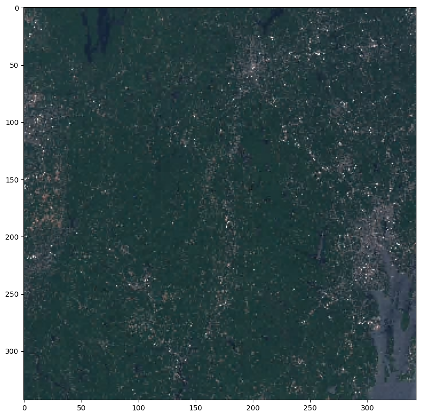
Each asset has a link which can be accessed from the href property. This can be a HTTP URL or a link to S3 for this STAC catalog. For example, let’s look at the link for the thumbnail of the scene.
print(assets["thumbnail"].href)
https://sentinel-cogs.s3.us-west-2.amazonaws.com/sentinel-s2-l2a-cogs/18/T/YM/2023/5/S2B_18TYM_20230527_0_L2A/thumbnail.jpg
Since this is a HTTP link, we can use Python requests package to load the image.
import requests
img_data = requests.get(assets["thumbnail"].href).content
import matplotlib.pyplot as plt
from PIL import Image
import io
plt.figure(figsize=(10, 10))
plt.imshow(Image.open(io.BytesIO(img_data)))
<matplotlib.image.AxesImage at 0xffff79a70520>
Now, let’s load one of the COG assets into memory. This is a large scene, and we don’t necessary want to load all the data at once. There are various packages to do this. Here we will use rioxarray, you can also use stacstack and odc-stac.
import rioxarray
nir_href = assets["nir"].href
nir = rioxarray.open_rasterio(nir_href)
nir
<xarray.DataArray (band: 1, y: 10980, x: 10980)>
[120560400 values with dtype=uint16]
Coordinates:
  * band         (band) int64 1
  * x            (x) float64 7e+05 7e+05 7e+05 ... 8.097e+05 8.097e+05 8.098e+05
  * y            (y) float64 4.7e+06 4.7e+06 4.7e+06 ... 4.59e+06 4.59e+06
    spatial_ref  int64 0
Attributes:
    AREA_OR_POINT:       Area
    OVR_RESAMPLING_ALG:  AVERAGE
    _FillValue:          0
    scale_factor:        1.0
add_offset: 0.0Note: At this stage the nir DataArray that we defined is empty, and only the metadata of the scene is loaded from the target href. This is consistent with open_rasterio function behavior, and you will learn more about it later in the class.
When you run any function on nir or call any of the built-in function (e.g. mean()) the data will be loaded to memory.
First, let’s plot part of the nir array.
import matplotlib.pyplot as plt
plt.imshow(nir[0,1500:2000,6200:7000], cmap='gray')
plt.clim(vmin=10, vmax=5000)
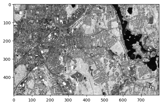
In this case, only the portion of the array that we wanted to visualize was loaded.
We can actually time the operation of plotting the whole scene vs the small portion we selected, and see the efficiency of using this approach.
%%timeit -n 5 -r 1
plt.imshow(nir[0,1500:2000,6200:7000], cmap='gray')
5.84 ms ± 0 ns per loop (mean ± std. dev. of 1 run, 5 loops each)
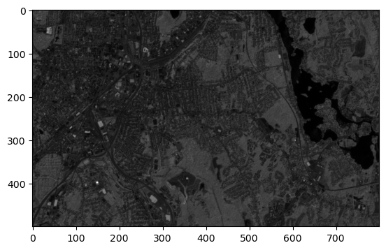
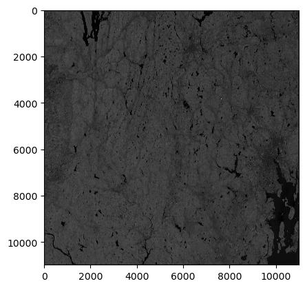
%%timeit -n 5 -r 1
plt.imshow(nir[0, :, :], cmap='gray')
43.2 s ± 0 ns per loop (mean ± std. dev. of 1 run, 5 loops each)
Lastly, you can save this array into a GeoTIFF file as following:
nir[0,1500:2000,6200:7000].rio.to_raster("nir_subset.tif")