10. Introduction to Dask#
Attribution: The following notebook is based on the great notebook created by Ryan Abernathey in the Earth and Environmental Data Science book (link)
10.1. What is Dask?#
Dask is a Python library that provides flexible parallel computing and distributed data processing capabilities. It is designed to handle larger-than-memory computations and parallelize tasks across multiple cores and even distributed clusters. Dask’s primary goal is to make it easier for developers to scale their data analysis and processing workflows while maintaining a familiar and Pythonic interface.
Dask is composed of two components: 1) Task Scheduler, and 2) “Big Data” collections. These collections include parallel arrays, dataframes, and lists that extend common interfaces like NumPy, Pandas, or Python iterators to larger-than-memory or distributed environments. These parallel collections run on top of dynamic task schedulers.

Dask overview (source: Dask Documentation)
10.2. Dask Arrays#
A dask array looks and feels a lot like a NumPy array. However, a dask array doesn’t directly hold any data. Instead, it symbolically represents the computations needed to generate the data. Nothing is actually computed until the actual numerical values are needed. This mode of operation is called “lazy”; it allows one to build up complex, large calculations symbolically before turning them over the scheduler for execution.
Dask arrays coordinate many NumPy arrays arranged into a grid. These arrays may live on disk or on other machines.

(source Dask Documentation)
If we want to create a NumPy array of all ones, we do it like this:
import numpy as np
shape = (1000, 4000)
ones_np = np.ones(shape)
ones_np
array([[1., 1., 1., ..., 1., 1., 1.],
       [1., 1., 1., ..., 1., 1., 1.],
       [1., 1., 1., ..., 1., 1., 1.],
       ...,
       [1., 1., 1., ..., 1., 1., 1.],
       [1., 1., 1., ..., 1., 1., 1.],
       [1., 1., 1., ..., 1., 1., 1.]])
This array contains ~ 30 MB of data:
ones_np.nbytes / (1024 * 1024)
30.517578125
Now let’s create the same array using dask’s array interface.
import dask.array as da
ones = da.ones(shape)
ones
|
||||||||||||||||
The dask array representation reveals the concept of “chunks”. “Chunks” describes how the array is split into sub-arrays. We did not specify any chunks, so Dask just used one single chunk for the array. This is not much different from a NumPy array at this point.
10.2.1. Specifying Chunks#
However, we could have split up the array into many chunks.
There are several ways to specify chunks. In this lecture, we will use a block shape.
chunk_shape = (1000, 1000)
ones = da.ones(shape, chunks=chunk_shape)
ones
|
||||||||||||||||
Notice that we just see a symbolic represetnation of the array, including its shape, dtype, and chunksize.
No data has been generated yet.
When we call .compute() on a dask array, the computation is trigger and the dask array becomes a NumPy array.
ones.compute()
array([[1., 1., 1., ..., 1., 1., 1.],
       [1., 1., 1., ..., 1., 1., 1.],
       [1., 1., 1., ..., 1., 1., 1.],
       ...,
       [1., 1., 1., ..., 1., 1., 1.],
       [1., 1., 1., ..., 1., 1., 1.],
       [1., 1., 1., ..., 1., 1., 1.]])
In order to understand what happened when we called .compute(), we can visualize the dask graph, the symbolic operations that make up the array
ones.visualize()
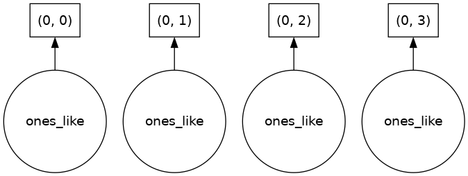
Our array has four chunks. To generate it, dask calls np.ones four times and then concatenates this together into one array.
Rather than immediately loading a dask array (which puts all the data into RAM), it is more common to want to reduce the data somehow. For example
sum_of_ones = ones.sum()
sum_of_ones.visualize()
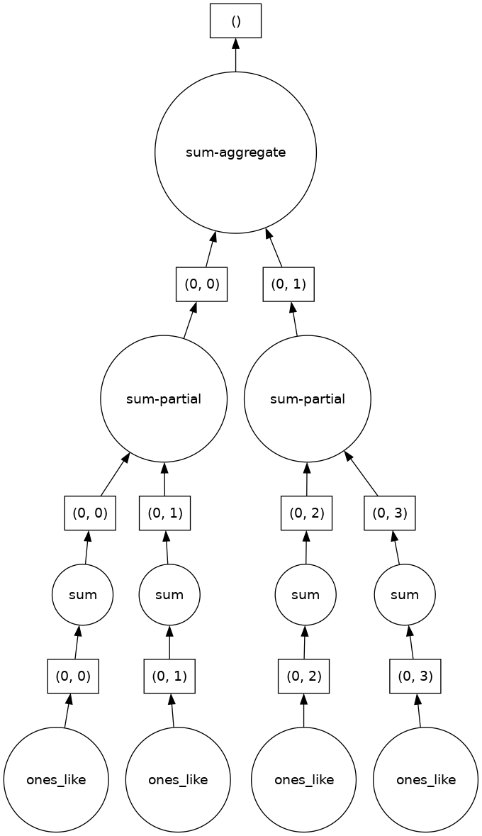
Here we see dask’s strategy for finding the sum. This simple example illustrates the beauty of dask: it automatically designs an algorithm appropriate for custom operations with big data.
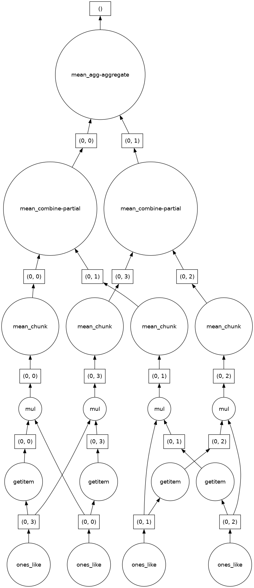
If we make our operation more complex, the graph gets more complex.
fancy_calculation = (ones * ones[::-1, ::-1]).mean()
fancy_calculation.visualize()
10.2.2. A Bigger Calculation#
The examples above were toy examples; the data (32 MB) is nowhere nearly big enough to warrant the use of dask.
We can make it a lot bigger!
bigshape = (200000, 4000)
big_ones = da.ones(bigshape, chunks=chunk_shape)
big_ones
|
||||||||||||||||
big_ones.nbytes / (1024 * 1024)
6103.515625
This dataset is 3.2 GB, rather MB! This is probably close to or greater than the amount of available RAM than you have in your computer. Nevertheless, dask has no problem working on it.
Do not try to .visualize() this array!
When doing a big calculation, dask also has some tools to help us understand what is happening under the hood
from dask.diagnostics import ProgressBar

big_calc = (big_ones * big_ones[::-1, ::-1]).mean()

with ProgressBar():
    result = big_calc.compute()
result
[########################################] | 100% Completed | 1.95 sms
1.0
10.2.3. Reduction#
All the usual NumPy methods work on dask arrays (Check this section on Dask Documentation to learn what NumPy methods work in Dask which ones don’t). You can also apply NumPy function directly to a dask array, and it will stay lazy.
big_ones_reduce = (np.cos(big_ones)**2).mean(axis=0)
big_ones_reduce
|
||||||||||||||||
Plotting also triggers computation, since we need the actual values
from matplotlib import pyplot as plt
%matplotlib inline
plt.rcParams['figure.figsize'] = (12,8)
plt.plot(big_ones_reduce)
[<matplotlib.lines.Line2D at 0x7f1d0d81fb10>]
10.3. Distributed Clusters#
Once we are ready to make a bigger calculation with dask, we can use a Dask Distributed cluster.
Warning
A common mistake is to move to distributed mode too soon. For smaller data, distributed will actually be much slower than the default multi-threaded scheduler or not using Dask at all. You should only use distributed when your data is much larger than what your computer can handle in memory.
10.3.1. Local Cluster#
A local cluster uses all the CPU cores of the machine it is running on. For our cloud-based Jupyterlab environments, that is just 2 cores–not very much. However, it’s good to know about.
from dask.distributed import Client, LocalCluster
cluster = LocalCluster()
client = Client(cluster)
client
Client
Client-a3b77291-5ee9-11ee-8693-6e1c11398774
| Connection method: Cluster object | Cluster type: distributed.LocalCluster |
| Dashboard: /user/halemohammad@clarku.edu/proxy/8787/status |
Cluster Info
LocalCluster
906ec967
| Dashboard: /user/halemohammad@clarku.edu/proxy/8787/status | Workers: 4 |
| Total threads: 8 | Total memory: 32.00 GiB |
| Status: running | Using processes: True |
Scheduler Info
Scheduler
Scheduler-6032ab8a-bce8-4aad-a8c7-c73352d67495
| Comm: tcp://127.0.0.1:38925 | Workers: 4 |
| Dashboard: /user/halemohammad@clarku.edu/proxy/8787/status | Total threads: 8 |
| Started: Just now | Total memory: 32.00 GiB |
Workers
Worker: 0
| Comm: tcp://127.0.0.1:46719 | Total threads: 2 |
| Dashboard: /user/halemohammad@clarku.edu/proxy/45657/status | Memory: 8.00 GiB |
| Nanny: tcp://127.0.0.1:41921 | |
| Local directory: /tmp/dask-scratch-space/worker-k38gkq3t | |
Worker: 1
| Comm: tcp://127.0.0.1:40449 | Total threads: 2 |
| Dashboard: /user/halemohammad@clarku.edu/proxy/37103/status | Memory: 8.00 GiB |
| Nanny: tcp://127.0.0.1:35223 | |
| Local directory: /tmp/dask-scratch-space/worker-3r0py63u | |
Worker: 2
| Comm: tcp://127.0.0.1:37551 | Total threads: 2 |
| Dashboard: /user/halemohammad@clarku.edu/proxy/35059/status | Memory: 8.00 GiB |
| Nanny: tcp://127.0.0.1:37127 | |
| Local directory: /tmp/dask-scratch-space/worker-7nyq_av7 | |
Worker: 3
| Comm: tcp://127.0.0.1:41805 | Total threads: 2 |
| Dashboard: /user/halemohammad@clarku.edu/proxy/40785/status | Memory: 8.00 GiB |
| Nanny: tcp://127.0.0.1:44145 | |
| Local directory: /tmp/dask-scratch-space/worker-6j58xfm7 | |
Note that the “Dashboard” link will open a new page where you can monitor a computation’s progress.
big_calc.compute()
1.0
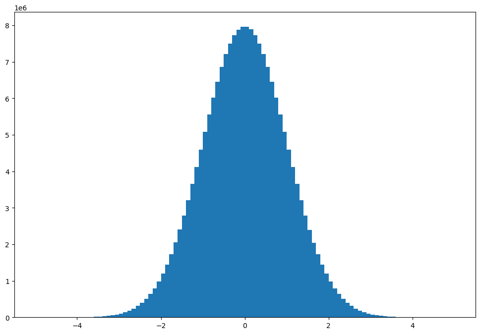
Here is another bigger calculation.
random_values = da.random.normal(size=(2e8,), chunks=(1e6,))
hist, bins = da.histogram(random_values, bins=100, range=[-5, 5])
hist
|
||||||||||||||||
# actually trigger the computation
hist_c = hist.compute()
# plot results
x = 0.5 * (bins[1:] + bins[:-1])
width = np.diff(bins)
plt.bar(x, hist_c, width);