7. Xarray Interpolation, Groupby, Resample, Rolling, and Coarsen#
Attribution: This notebook is a revision of the Xarray Interpolation, Groupby, Resample, Rolling, and Coarsen notebook by Ryan Abernathey from An Introduction to Earth and Environmental Data Science. Thanks to Aiyin Zhang for preparing this notebook.
In this lesson, we cover some more advanced aspects of xarray.
You can access this notebook (in a Docker image) on this GitHub repo.
import numpy as np
import xarray as xr
from matplotlib import pyplot as plt
7.1. Interpolation#
In the previous lesson on xarray, we learned how to select data based on its dimension coordinates and align data with dimension different coordinates.
But what if we want to estimate the value of the data variables at different coordinates.
This is where interpolation comes in.
# we write it out explicitly so we can see each point.
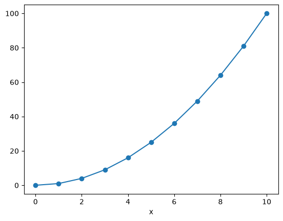
x_data = np.array([0, 1, 2, 3, 4, 5, 6, 7, 8, 9, 10])
f = xr.DataArray(x_data**2, dims=['x'], coords={'x': x_data})
f
<xarray.DataArray (x: 11)> Size: 88B
array([  0,   1,   4,   9,  16,  25,  36,  49,  64,  81, 100])
Coordinates:
  * x        (x) int64 88B 0 1 2 3 4 5 6 7 8 9 10
f.plot(marker='o')
[<matplotlib.lines.Line2D at 0x146e902d0>]
f.sel(x=3)
<xarray.DataArray ()> Size: 8B
array(9)
Coordinates:
x int64 8B 3We only have data on the integer points in x. But what if we wanted to estimate the value at, say, 4.5?
f.sel(x=4.5)
---------------------------------------------------------------------------
KeyError                                  Traceback (most recent call last)
File ~/Desktop/xarray-tutorial/.pixi/envs/default/lib/python3.13/site-packages/pandas/core/indexes/base.py:3641, in Index.get_loc(self, key)
   3640 try:
-> 3641     return self._engine.get_loc(casted_key)
   3642 except KeyError as err:

File pandas/_libs/index.pyx:168, in pandas._libs.index.IndexEngine.get_loc()
--> 168 'Could not get source, probably due dynamically evaluated source code.'

File pandas/_libs/index.pyx:176, in pandas._libs.index.IndexEngine.get_loc()
--> 176 'Could not get source, probably due dynamically evaluated source code.'

File pandas/_libs/index_class_helper.pxi:70, in pandas._libs.index.Int64Engine._check_type()
---> 70 'Could not get source, probably due dynamically evaluated source code.'

KeyError: 4.5

The above exception was the direct cause of the following exception:

KeyError                                  Traceback (most recent call last)
File ~/Desktop/xarray-tutorial/.pixi/envs/default/lib/python3.13/site-packages/xarray/core/indexes.py:878, in PandasIndex.sel(self, labels, method, tolerance)
    877 try:
--> 878     indexer = self.index.get_loc(label_value)
    879 except KeyError as e:

File ~/Desktop/xarray-tutorial/.pixi/envs/default/lib/python3.13/site-packages/pandas/core/indexes/base.py:3648, in Index.get_loc(self, key)
   3647         raise InvalidIndexError(key) from err
-> 3648     raise KeyError(key) from err
   3649 except TypeError:
   3650     # If we have a listlike key, _check_indexing_error will raise
   3651     #  InvalidIndexError. Otherwise we fall through and re-raise
   3652     #  the TypeError.

KeyError: 4.5

The above exception was the direct cause of the following exception:

KeyError                                  Traceback (most recent call last)
Cell In[5], line 1
----> 1 f.sel(x=4.5)

File ~/Desktop/xarray-tutorial/.pixi/envs/default/lib/python3.13/site-packages/xarray/core/dataarray.py:1729, in DataArray.sel(self, indexers, method, tolerance, drop, **indexers_kwargs)
   1613 def sel(
   1614     self,
   1615     indexers: Mapping[Any, Any] | None = None,
   (...)   1619     **indexers_kwargs: Any,
   1620 ) -> Self:
   1621     """Return a new DataArray whose data is given by selecting index
   1622     labels along the specified dimension(s).
   1623
   (...)   1727     Dimensions without coordinates: points
   1728     """
-> 1729     ds = self._to_temp_dataset().sel(
   1730         indexers=indexers,
   1731         drop=drop,
   1732         method=method,
   1733         tolerance=tolerance,
   1734         **indexers_kwargs,
   1735     )
   1736     return self._from_temp_dataset(ds)

File ~/Desktop/xarray-tutorial/.pixi/envs/default/lib/python3.13/site-packages/xarray/core/dataset.py:3073, in Dataset.sel(self, indexers, method, tolerance, drop, **indexers_kwargs)
   3069             Tutorial material on basics of indexing
   3070
   3071         """
   3072         indexers = either_dict_or_kwargs(indexers, indexers_kwargs, "sel")
-> 3073         query_results = map_index_queries(
   3074             self, indexers=indexers, method=method, tolerance=tolerance
   3075         )
   3076

File ~/Desktop/xarray-tutorial/.pixi/envs/default/lib/python3.13/site-packages/xarray/core/indexing.py:219, in map_index_queries(obj, indexers, method, tolerance, **indexers_kwargs)
    217         results.append(IndexSelResult(labels))
    218     else:
--> 219         results.append(index.sel(labels, **options))
    221 merged = merge_sel_results(results)
    223 # drop dimension coordinates found in dimension indexers
    224 # (also drop multi-index if any)
    225 # (.sel() already ensures alignment)

File ~/Desktop/xarray-tutorial/.pixi/envs/default/lib/python3.13/site-packages/xarray/core/indexes.py:880, in PandasIndex.sel(self, labels, method, tolerance)
    878             indexer = self.index.get_loc(label_value)
    879         except KeyError as e:
--> 880             raise KeyError(
    881                 f"not all values found in index {coord_name!r}. "
    882                 "Try setting the `method` keyword argument (example: method='nearest')."
    883             ) from e
    885 elif label_array.dtype.kind == "b":
    886     indexer = label_array

KeyError: "not all values found in index 'x'. Try setting the `method` keyword argument (example: method='nearest')."
Interpolation to the rescue!
f.interp(x=4.5)
<xarray.DataArray ()> Size: 8B
array(20.5)
Coordinates:
x float64 8B 4.5Interpolation uses scipy.interpolate under the hood. There are different modes of interpolation.
f.interp(x=4.5, method='linear').values
array(20.5)
f.interp(x=4.5, method='nearest').values
array(16.)
f.interp(x=4.5, method='cubic').values
array(20.25)
We can interpolate to a whole new set of coordinates at once:
x_new = x_data + 0.5
f_interp_linear = f.interp(x=x_new, method='linear')
f_interp_cubic = f.interp(x=x_new, method='cubic')
f.plot(marker='o', label='original')
f_interp_linear.plot(marker='o', label='linear')
f_interp_cubic.plot(marker='o', label='cubic')
plt.legend()
<matplotlib.legend.Legend at 0x14703b4d0>
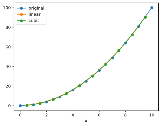
Note that values outside of the original range are not supported:
f_interp_cubic.values
array([ 0.25,  2.25,  6.25, 12.25, 20.25, 30.25, 42.25, 56.25, 72.25,
       90.25,   nan])
Note
You can apply interpolation to any dimension, and even to multiple dimensions at a time.
(Multidimensional interpolation only supports mode='nearest' and mode='linear'.)
But keep in mind that xarray has no built-in understanding of geography.
If you use interp on lat / lon coordinates, it will just perform naive interpolation of the lat / lon values.
More sophisticated treatment of spherical geometry requires another package such as xesmf.
7.2. Loading Data from NetCDF Files#
NetCDF (Network Common Data Format) is the most widely used format for distributing geoscience data. NetCDF is maintained by the Unidata organization.
Below we quote from the NetCDF website:
NetCDF (network Common Data Form) is a set of interfaces for array-oriented data access and a freely distributed collection of data access libraries for C, Fortran, C++, Java, and other languages. The netCDF libraries support a machine-independent format for representing scientific data. Together, the interfaces, libraries, and format support the creation, access, and sharing of scientific data.
NetCDF data is:
Self-Describing. A netCDF file includes information about the data it contains.
Portable. A netCDF file can be accessed by computers with different ways of storing integers, characters, and floating-point numbers.
Scalable. A small subset of a large dataset may be accessed efficiently.
Appendable. Data may be appended to a properly structured netCDF file without copying the dataset or redefining its structure.
Sharable. One writer and multiple readers may simultaneously access the same netCDF file.
Archivable. Access to all earlier forms of netCDF data will be supported by current and future versions of the software.
xarray is designed to make reading netCDF files in python as easy, powerful, and flexible as possible. (See xarray netCDF docs for more details.)
Below we download and load some the NASA GISSTemp global temperature anomaly dataset. The original file is located at https://data.giss.nasa.gov/pub/gistemp/gistemp1200_GHCNv4_ERSSTv5.nc.gz.
import pooch
gis_temp_url = 'https://data.giss.nasa.gov/pub/gistemp/gistemp1200_GHCNv4_ERSSTv5.nc.gz'

gis_temp_file = pooch.retrieve(
    gis_temp_url,
    processor=pooch.Decompress(),
    known_hash="6a597332bcefbe0fbe5a6ce7677a9012fa766cc43cea291d6207c12db2fe0cc6"
)
gis_temp = xr.open_dataset(gis_temp_file)
gis_temp
<xarray.Dataset> Size: 114MB
Dimensions:      (time: 1760, nv: 2, lat: 90, lon: 180)
Coordinates:
  * time         (time) datetime64[ns] 14kB 1880-01-15 1880-02-15 ... 2026-08-15
  * lat          (lat) float32 360B -89.0 -87.0 -85.0 -83.0 ... 85.0 87.0 89.0
  * lon          (lon) float32 720B -179.0 -177.0 -175.0 ... 175.0 177.0 179.0
Dimensions without coordinates: nv
Data variables:
    time_bnds    (time, nv) datetime64[ns] 28kB ...
    tempanomaly  (time, lat, lon) float32 114MB ...
Attributes:
    title:        GISTEMP Surface Temperature Analysis
    institution:  NASA Goddard Institute for Space Studies
    source:       http://data.giss.nasa.gov/gistemp/
    Conventions:  CF-1.6
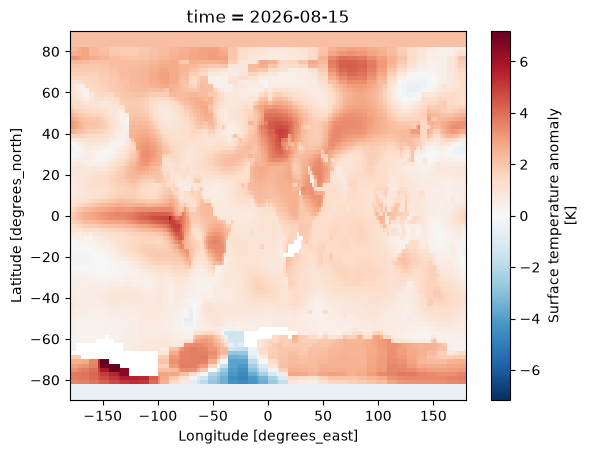
history: Created 2026-09-08 02:31:15 by SBBX_to_nc 2.0 - ILAND=1200,...gis_temp.tempanomaly.isel(time=-1).plot()
plt.show()
gis_temp.tempanomaly.mean(dim=('lon', 'lat')).plot()
plt.show()
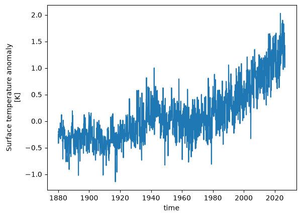
Let’s visualize the temperature anomally for the grid near Worcester. (Worcester’s coordinates: latitude: 42.2626; longtitude: -71.8023)
gis_temp.tempanomaly.sel(lat=42.2626, lon=-71.8023, method='nearest').plot()
plt.show()
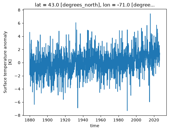
Note that you need to define method since the corresponding values for Worcester latitude and longitude do not exist in the DataArray’s coordinates.
7.3. Groupby#
xarray copies pandas' very useful groupby functionality, enabling the “split / apply / combine” workflow on xarray DataArrays and Datasets. In the first part of the lesson, we will learn to use groupby by analyzing sea-surface temperature data.
First we load a dataset. We will use the NOAA Extended Reconstructed Sea Surface Temperature (ERSST) v5 product, a widely used and trusted gridded compilation of historical data going back to 1854.
Since the data is provided via an OPeNDAP server, we can load it directly without downloading anything:
The code to this would have been:
noaa_sst_url = 'https://psl.noaa.gov/thredds/fileServer/Datasets/noaa.ersst.v6/sst.mnmean.nc'
noaa_sst = xr.open_dataset(noaa_sst_url, drop_variables=['time_bnds'])
Unfortunately, as of September 2026, NOAA is updating their data servers and the connection to retrieve the file breaks. This results in the xarray package not being able to retrieve the data. So, we have added the same NetCDF file to the course website for easy access.
noaa_sst_url = 'https://raw.githubusercontent.com/HamedAlemo/advanced-geo-python/main/files/noaa.ersst.v6/sst.mnmean.nc'

noaa_sst_file = pooch.retrieve(
    noaa_sst_url,
    known_hash="ef61d97774bda4cc21324a8ce33059ac826101590c0da9911ec1ceb8bcf357b7"
)
noaa_sst = xr.open_dataset(noaa_sst_file, drop_variables=['time_bnds'])
noaa_sst = noaa_sst.sel(time=slice('1960', '2025'))
noaa_sst
<xarray.Dataset> Size: 51MB
Dimensions:  (time: 792, lat: 89, lon: 180)
Coordinates:
  * time     (time) datetime64[ns] 6kB 1960-01-01 1960-02-01 ... 2025-12-01
  * lat      (lat) float32 356B 88.0 86.0 84.0 82.0 ... -82.0 -84.0 -86.0 -88.0
  * lon      (lon) float32 720B 0.0 2.0 4.0 6.0 8.0 ... 352.0 354.0 356.0 358.0
Data variables:
    sst      (time, lat, lon) float32 51MB ...
Attributes: (12/39)
    climatology:               Climatology is based on 1971-2000 SST, Xue, Y....
    description:               In situ data: ICOADS2.5 before 2007 and NCEP i...
    keywords_vocabulary:       NASA Global Change Master Directory (GCMD) Sci...
    keywords:                  Earth Science > Oceans > Ocean Temperature > S...
    instrument:                Conventional thermometers
    source_comment:            SSTs were observed by conventional thermometer...
    ...                        ...
    product_version:           Version 6
    history:                   created 01/16/2025 by PSL using NCEI ERSST V6 ...
    References:                https://www.ncdc.noaa.gov/data-access/marineoc...
    summary:                   ERSSTv6 is developped based on v5, by replacin...
    comments:                  SSTs were observed by conventional thermometer...
platform: Ship and Buoy SSTs from ICOADS R3.0.2 and Argo...Let’s do some basic visualizations of the data, just to make sure it looks reasonable.
fig, ax = plt.subplots()
noaa_sst.sst.sel(time = '2025-01-01').plot(ax=ax, vmin=-2, vmax=30)
plt.show()
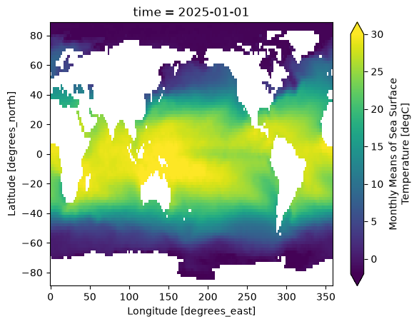
Note that xarray correctly parsed the time index, resulting in a Pandas datetime index on the time dimension.
noaa_sst.time
<xarray.DataArray 'time' (time: 792)> Size: 6kB
array(['1960-01-01T00:00:00.000000000', '1960-02-01T00:00:00.000000000',
       '1960-03-01T00:00:00.000000000', ..., '2025-10-01T00:00:00.000000000',
       '2025-11-01T00:00:00.000000000', '2025-12-01T00:00:00.000000000'],
      shape=(792,), dtype='datetime64[ns]')
Coordinates:
* time (time) datetime64[ns] 6kB 1960-01-01 1960-02-01 ... 2025-12-01
Attributes:
long_name: Time
delta_t: 0000-01-00 00:00:00
avg_period: 0000-01-00 00:00:00
prev_avg_period: 0000-00-07 00:00:00
standard_name: time
axis: T
actual_range: [18262. 82757.]noaa_sst.sst.sel(lon=300, lat=50).plot()
plt.show()
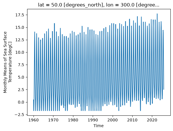
As we can see from the plot, the timeseries at any one point is totally dominated by the seasonal cycle. We would like to remove this seasonal cycle (called the “climatology”) in order to better see the long-term variaitions in temperature. We will accomplish this using groupby.
The syntax of xarray’s groupby is almost identical to pandas.
We will first apply groupby to a single DataArray.
7.3.1. Split Step#
The most important argument is group: this defines the unique values we will use to “split” the data for grouped analysis. We can pass either a DataArray or a name of a variable in the dataset. Lets first use a DataArray. Just like with pandas, we can use the time index to extract specific components of dates and times. xarray uses a special syntax for this .dt, called the DatetimeAccessor.
See a list of datatime properties you can access through .dt here
noaa_sst.time.dt
<xarray.core.accessor_dt.DatetimeAccessor at 0x175158810>
noaa_sst.time.dt.month
<xarray.DataArray 'month' (time: 792)> Size: 6kB
array([ 1,  2,  3,  4,  5,  6,  7,  8,  9, 10, 11, 12,  1,  2,  3,  4,  5,
        6,  7,  8,  9, 10, 11, 12,  1,  2,  3,  4,  5,  6,  7,  8,  9, 10,
       11, 12,  1,  2,  3,  4,  5,  6,  7,  8,  9, 10, 11, 12,  1,  2,  3,
        4,  5,  6,  7,  8,  9, 10, 11, 12,  1,  2,  3,  4,  5,  6,  7,  8,
        9, 10, 11, 12,  1,  2,  3,  4,  5,  6,  7,  8,  9, 10, 11, 12,  1,
        2,  3,  4,  5,  6,  7,  8,  9, 10, 11, 12,  1,  2,  3,  4,  5,  6,
        7,  8,  9, 10, 11, 12,  1,  2,  3,  4,  5,  6,  7,  8,  9, 10, 11,
       12,  1,  2,  3,  4,  5,  6,  7,  8,  9, 10, 11, 12,  1,  2,  3,  4,
        5,  6,  7,  8,  9, 10, 11, 12,  1,  2,  3,  4,  5,  6,  7,  8,  9,
       10, 11, 12,  1,  2,  3,  4,  5,  6,  7,  8,  9, 10, 11, 12,  1,  2,
        3,  4,  5,  6,  7,  8,  9, 10, 11, 12,  1,  2,  3,  4,  5,  6,  7,
        8,  9, 10, 11, 12,  1,  2,  3,  4,  5,  6,  7,  8,  9, 10, 11, 12,
        1,  2,  3,  4,  5,  6,  7,  8,  9, 10, 11, 12,  1,  2,  3,  4,  5,
        6,  7,  8,  9, 10, 11, 12,  1,  2,  3,  4,  5,  6,  7,  8,  9, 10,
       11, 12,  1,  2,  3,  4,  5,  6,  7,  8,  9, 10, 11, 12,  1,  2,  3,
        4,  5,  6,  7,  8,  9, 10, 11, 12,  1,  2,  3,  4,  5,  6,  7,  8,
        9, 10, 11, 12,  1,  2,  3,  4,  5,  6,  7,  8,  9, 10, 11, 12,  1,
        2,  3,  4,  5,  6,  7,  8,  9, 10, 11, 12,  1,  2,  3,  4,  5,  6,
        7,  8,  9, 10, 11, 12,  1,  2,  3,  4,  5,  6,  7,  8,  9, 10, 11,
       12,  1,  2,  3,  4,  5,  6,  7,  8,  9, 10, 11, 12,  1,  2,  3,  4,
...
        4,  5,  6,  7,  8,  9, 10, 11, 12,  1,  2,  3,  4,  5,  6,  7,  8,
        9, 10, 11, 12,  1,  2,  3,  4,  5,  6,  7,  8,  9, 10, 11, 12,  1,
        2,  3,  4,  5,  6,  7,  8,  9, 10, 11, 12,  1,  2,  3,  4,  5,  6,
        7,  8,  9, 10, 11, 12,  1,  2,  3,  4,  5,  6,  7,  8,  9, 10, 11,
       12,  1,  2,  3,  4,  5,  6,  7,  8,  9, 10, 11, 12,  1,  2,  3,  4,
        5,  6,  7,  8,  9, 10, 11, 12,  1,  2,  3,  4,  5,  6,  7,  8,  9,
       10, 11, 12,  1,  2,  3,  4,  5,  6,  7,  8,  9, 10, 11, 12,  1,  2,
        3,  4,  5,  6,  7,  8,  9, 10, 11, 12,  1,  2,  3,  4,  5,  6,  7,
        8,  9, 10, 11, 12,  1,  2,  3,  4,  5,  6,  7,  8,  9, 10, 11, 12,
        1,  2,  3,  4,  5,  6,  7,  8,  9, 10, 11, 12,  1,  2,  3,  4,  5,
        6,  7,  8,  9, 10, 11, 12,  1,  2,  3,  4,  5,  6,  7,  8,  9, 10,
       11, 12,  1,  2,  3,  4,  5,  6,  7,  8,  9, 10, 11, 12,  1,  2,  3,
        4,  5,  6,  7,  8,  9, 10, 11, 12,  1,  2,  3,  4,  5,  6,  7,  8,
        9, 10, 11, 12,  1,  2,  3,  4,  5,  6,  7,  8,  9, 10, 11, 12,  1,
        2,  3,  4,  5,  6,  7,  8,  9, 10, 11, 12,  1,  2,  3,  4,  5,  6,
        7,  8,  9, 10, 11, 12,  1,  2,  3,  4,  5,  6,  7,  8,  9, 10, 11,
       12,  1,  2,  3,  4,  5,  6,  7,  8,  9, 10, 11, 12,  1,  2,  3,  4,
        5,  6,  7,  8,  9, 10, 11, 12,  1,  2,  3,  4,  5,  6,  7,  8,  9,
       10, 11, 12,  1,  2,  3,  4,  5,  6,  7,  8,  9, 10, 11, 12,  1,  2,
        3,  4,  5,  6,  7,  8,  9, 10, 11, 12])
Coordinates:
  * time     (time) datetime64[ns] 6kB 1960-01-01 1960-02-01 ... 2025-12-01
Attributes:
    long_name:        Time
    delta_t:          0000-01-00 00:00:00
    avg_period:       0000-01-00 00:00:00
    prev_avg_period:  0000-00-07 00:00:00
    standard_name:    time
    axis:             T
actual_range: [18262. 82757.]noaa_sst.time.dt.year
<xarray.DataArray 'year' (time: 792)> Size: 6kB
array([1960, 1960, 1960, 1960, 1960, 1960, 1960, 1960, 1960, 1960, 1960,
       1960, 1961, 1961, 1961, 1961, 1961, 1961, 1961, 1961, 1961, 1961,
       1961, 1961, 1962, 1962, 1962, 1962, 1962, 1962, 1962, 1962, 1962,
       1962, 1962, 1962, 1963, 1963, 1963, 1963, 1963, 1963, 1963, 1963,
       1963, 1963, 1963, 1963, 1964, 1964, 1964, 1964, 1964, 1964, 1964,
       1964, 1964, 1964, 1964, 1964, 1965, 1965, 1965, 1965, 1965, 1965,
       1965, 1965, 1965, 1965, 1965, 1965, 1966, 1966, 1966, 1966, 1966,
       1966, 1966, 1966, 1966, 1966, 1966, 1966, 1967, 1967, 1967, 1967,
       1967, 1967, 1967, 1967, 1967, 1967, 1967, 1967, 1968, 1968, 1968,
       1968, 1968, 1968, 1968, 1968, 1968, 1968, 1968, 1968, 1969, 1969,
       1969, 1969, 1969, 1969, 1969, 1969, 1969, 1969, 1969, 1969, 1970,
       1970, 1970, 1970, 1970, 1970, 1970, 1970, 1970, 1970, 1970, 1970,
       1971, 1971, 1971, 1971, 1971, 1971, 1971, 1971, 1971, 1971, 1971,
       1971, 1972, 1972, 1972, 1972, 1972, 1972, 1972, 1972, 1972, 1972,
       1972, 1972, 1973, 1973, 1973, 1973, 1973, 1973, 1973, 1973, 1973,
       1973, 1973, 1973, 1974, 1974, 1974, 1974, 1974, 1974, 1974, 1974,
       1974, 1974, 1974, 1974, 1975, 1975, 1975, 1975, 1975, 1975, 1975,
       1975, 1975, 1975, 1975, 1975, 1976, 1976, 1976, 1976, 1976, 1976,
       1976, 1976, 1976, 1976, 1976, 1976, 1977, 1977, 1977, 1977, 1977,
       1977, 1977, 1977, 1977, 1977, 1977, 1977, 1978, 1978, 1978, 1978,
...
       2007, 2007, 2007, 2007, 2008, 2008, 2008, 2008, 2008, 2008, 2008,
       2008, 2008, 2008, 2008, 2008, 2009, 2009, 2009, 2009, 2009, 2009,
       2009, 2009, 2009, 2009, 2009, 2009, 2010, 2010, 2010, 2010, 2010,
       2010, 2010, 2010, 2010, 2010, 2010, 2010, 2011, 2011, 2011, 2011,
       2011, 2011, 2011, 2011, 2011, 2011, 2011, 2011, 2012, 2012, 2012,
       2012, 2012, 2012, 2012, 2012, 2012, 2012, 2012, 2012, 2013, 2013,
       2013, 2013, 2013, 2013, 2013, 2013, 2013, 2013, 2013, 2013, 2014,
       2014, 2014, 2014, 2014, 2014, 2014, 2014, 2014, 2014, 2014, 2014,
       2015, 2015, 2015, 2015, 2015, 2015, 2015, 2015, 2015, 2015, 2015,
       2015, 2016, 2016, 2016, 2016, 2016, 2016, 2016, 2016, 2016, 2016,
       2016, 2016, 2017, 2017, 2017, 2017, 2017, 2017, 2017, 2017, 2017,
       2017, 2017, 2017, 2018, 2018, 2018, 2018, 2018, 2018, 2018, 2018,
       2018, 2018, 2018, 2018, 2019, 2019, 2019, 2019, 2019, 2019, 2019,
       2019, 2019, 2019, 2019, 2019, 2020, 2020, 2020, 2020, 2020, 2020,
       2020, 2020, 2020, 2020, 2020, 2020, 2021, 2021, 2021, 2021, 2021,
       2021, 2021, 2021, 2021, 2021, 2021, 2021, 2022, 2022, 2022, 2022,
       2022, 2022, 2022, 2022, 2022, 2022, 2022, 2022, 2023, 2023, 2023,
       2023, 2023, 2023, 2023, 2023, 2023, 2023, 2023, 2023, 2024, 2024,
       2024, 2024, 2024, 2024, 2024, 2024, 2024, 2024, 2024, 2024, 2025,
       2025, 2025, 2025, 2025, 2025, 2025, 2025, 2025, 2025, 2025, 2025])
Coordinates:
  * time     (time) datetime64[ns] 6kB 1960-01-01 1960-02-01 ... 2025-12-01
Attributes:
    long_name:        Time
    delta_t:          0000-01-00 00:00:00
    avg_period:       0000-01-00 00:00:00
    prev_avg_period:  0000-00-07 00:00:00
    standard_name:    time
    axis:             T
actual_range: [18262. 82757.]We can use these arrays in a groupby operation:
gb = noaa_sst.sst.groupby(noaa_sst.time.dt.month)
gb
<DataArrayGroupBy, grouped over 1 grouper(s), 12 groups in total:
    'month': UniqueGrouper('month'), 12/12 groups with labels 1, 2, 3, 4, 5, 6, 7, 8, 9, 10, 11, 12>
xarray also offers a more concise syntax when the variable you’re grouping on is already present in the dataset. This is identical to the previous line:
gb = noaa_sst.sst.groupby('time.month')
gb
<DataArrayGroupBy, grouped over 1 grouper(s), 12 groups in total:
    'month': UniqueGrouper('month'), 12/12 groups with labels 1, 2, 3, 4, 5, 6, 7, 8, 9, 10, 11, 12>
Now that the data are split, we can manually iterate over the group. The iterator returns the key (group name) and the value (the actual dataset corresponding to that group) for each group.
for group_name, group_da in gb:
    print(group_name) # stop after first iteration
    break
group_da
1
<xarray.DataArray 'sst' (time: 66, lat: 89, lon: 180)> Size: 4MB
[1057320 values with dtype=float32]
Coordinates:
  * time     (time) datetime64[ns] 528B 1960-01-01 1961-01-01 ... 2025-01-01
  * lat      (lat) float32 356B 88.0 86.0 84.0 82.0 ... -82.0 -84.0 -86.0 -88.0
  * lon      (lon) float32 720B 0.0 2.0 4.0 6.0 8.0 ... 352.0 354.0 356.0 358.0
Attributes:
    long_name:     Monthly Means of Sea Surface Temperature
    units:         degC
    var_desc:      Sea Surface Temperature
    level_desc:    Surface
    statistic:     Mean
    parent_stat:   Individual Values
    valid_range:   [-1.8 45. ]
    actual_range:  [-2.2655034 42.32636  ]
dataset: NOAA Extended Reconstructed SST V67.3.2. Map & Combine#
Now that we have groups defined, it’s time to “apply” a calculation to the group. Like in pandas, these calculations can either be:
aggregation: reduces the size of the group
transformation: preserves the group’s full size
At then end of the apply step, xarray will automatically combine the aggregated / transformed groups back into a single object.
Warning
Xarray calls the “apply” step map. This is different from Pandas!
gb.map?
Signature:
gb.map(
    func: 'Callable[..., DataArray]',
    args: 'tuple[Any, ...]' = (),
    shortcut: 'bool | None' = None,
    **kwargs: 'Any',
) -> 'DataArray'
Docstring:
Apply a function to each array in the group and concatenate them
together into a new array.

`func` is called like `func(ar, *args, **kwargs)` for each array `ar`
in this group.

Apply uses heuristics (like `pandas.GroupBy.apply`) to figure out how
to stack together the array. The rule is:

1. If the dimension along which the group coordinate is defined is
   still in the first grouped array after applying `func`, then stack
   over this dimension.
2. Otherwise, stack over the new dimension given by name of this
   grouping (the argument to the `groupby` function).

Parameters
----------
func : callable
    Callable to apply to each array.
shortcut : bool, optional
    Whether or not to shortcut evaluation under the assumptions that:

    (1) The action of `func` does not depend on any of the array
        metadata (attributes or coordinates) but only on the data and
        dimensions.
    (2) The action of `func` creates arrays with homogeneous metadata,
        that is, with the same dimensions and attributes.

    If these conditions are satisfied `shortcut` provides significant
    speedup. This should be the case for many common groupby operations
    (e.g., applying numpy ufuncs).
*args : tuple, optional
    Positional arguments passed to `func`.
**kwargs
    Used to call `func(ar, **kwargs)` for each array `ar`.

Returns
-------
applied : DataArray
    The result of splitting, applying and combining this array.
File:      ~/Desktop/xarray-tutorial/.pixi/envs/default/lib/python3.13/site-packages/xarray/core/groupby.py
Type:      method
7.3.2.1. Aggregations#
Like pandas, xarray’s groupby object has many built-in aggregation operations (e.g. mean, min, max, std, etc):
sst_mm = gb.mean(dim='time')
sst_mm
<xarray.DataArray 'sst' (month: 12, lat: 89, lon: 180)> Size: 769kB
array([[[-1.7704183, -1.7429352, -1.7334596, ..., -1.7583696,
         -1.7611848, -1.7661368],
        [-1.7474002, -1.72093  , -1.7083223, ..., -1.6872082,
         -1.679056 , -1.7087934],
        [-1.7070372, -1.6970297, -1.717903 , ..., -1.7212163,
         -1.7391362, -1.739069 ],
        ...,
        [       nan,        nan,        nan, ...,        nan,
                nan,        nan],
        [       nan,        nan,        nan, ...,        nan,
                nan,        nan],
        [       nan,        nan,        nan, ...,        nan,
                nan,        nan]],

       [[-1.7687984, -1.7444975, -1.7376387, ..., -1.7793446,
         -1.7700444, -1.7667769],
        [-1.7611471, -1.7221469, -1.7059942, ..., -1.7024916,
         -1.6803567, -1.7156144],
        [-1.7125304, -1.6979598, -1.7094287, ..., -1.7250212,
         -1.739435 , -1.7409368],
...
        [       nan,        nan,        nan, ...,        nan,
                nan,        nan],
        [       nan,        nan,        nan, ...,        nan,
                nan,        nan],
        [       nan,        nan,        nan, ...,        nan,
                nan,        nan]],

       [[-1.7231394, -1.6888553, -1.6701957, ..., -1.7321169,
         -1.7216377, -1.7196321],
        [-1.6872448, -1.674    , -1.6818368, ..., -1.6700076,
         -1.6486129, -1.6574895],
        [-1.6927167, -1.6861418, -1.7194597, ..., -1.7171193,
         -1.7197195, -1.7169719],
        ...,
        [       nan,        nan,        nan, ...,        nan,
                nan,        nan],
        [       nan,        nan,        nan, ...,        nan,
                nan,        nan],
        [       nan,        nan,        nan, ...,        nan,
                nan,        nan]]], shape=(12, 89, 180), dtype=float32)
Coordinates:
  * month    (month) int64 96B 1 2 3 4 5 6 7 8 9 10 11 12
  * lat      (lat) float32 356B 88.0 86.0 84.0 82.0 ... -82.0 -84.0 -86.0 -88.0
  * lon      (lon) float32 720B 0.0 2.0 4.0 6.0 8.0 ... 352.0 354.0 356.0 358.0
Attributes:
    long_name:     Monthly Means of Sea Surface Temperature
    units:         degC
    var_desc:      Sea Surface Temperature
    level_desc:    Surface
    statistic:     Mean
    parent_stat:   Individual Values
    valid_range:   [-1.8 45. ]
    actual_range:  [-2.2655034 42.32636  ]
dataset: NOAA Extended Reconstructed SST V6.map accepts as its argument a function. We can pass an existing function:
gb.map(np.mean)
<xarray.DataArray 'sst' (month: 12)> Size: 48B
array([13.628319 , 13.7344055, 13.726181 , 13.641603 , 13.591497 ,
13.660077 , 13.876824 , 14.041093 , 13.923461 , 13.645469 ,
13.463244 , 13.489468 ], dtype=float32)
Coordinates:
* month (month) int64 96B 1 2 3 4 5 6 7 8 9 10 11 12
Attributes:
long_name: Monthly Means of Sea Surface Temperature
units: degC
var_desc: Sea Surface Temperature
level_desc: Surface
statistic: Mean
parent_stat: Individual Values
valid_range: [-1.8 45. ]
actual_range: [-2.2655034 42.32636 ]
dataset: NOAA Extended Reconstructed SST V6Because we specified no extra arguments (like axis) the function was applied over all space and time dimensions. This is not what we wanted. Instead, we could define a custom function. This function takes a single argument –the group dataset– and returns a new dataset to be combined:
def time_mean(a):
return a.mean(dim='time')
sst_mm = gb.map(time_mean)
sst_mm
<xarray.DataArray 'sst' (month: 12, lat: 89, lon: 180)> Size: 769kB
array([[[-1.7704183, -1.7429352, -1.7334596, ..., -1.7583696,
         -1.7611848, -1.7661368],
        [-1.7474002, -1.72093  , -1.7083223, ..., -1.6872082,
         -1.679056 , -1.7087934],
        [-1.7070372, -1.6970297, -1.717903 , ..., -1.7212163,
         -1.7391362, -1.739069 ],
        ...,
        [       nan,        nan,        nan, ...,        nan,
                nan,        nan],
        [       nan,        nan,        nan, ...,        nan,
                nan,        nan],
        [       nan,        nan,        nan, ...,        nan,
                nan,        nan]],

       [[-1.7687984, -1.7444975, -1.7376387, ..., -1.7793446,
         -1.7700444, -1.7667769],
        [-1.7611471, -1.7221469, -1.7059942, ..., -1.7024916,
         -1.6803567, -1.7156144],
        [-1.7125304, -1.6979598, -1.7094287, ..., -1.7250212,
         -1.739435 , -1.7409368],
...
        [       nan,        nan,        nan, ...,        nan,
                nan,        nan],
        [       nan,        nan,        nan, ...,        nan,
                nan,        nan],
        [       nan,        nan,        nan, ...,        nan,
                nan,        nan]],

       [[-1.7231394, -1.6888553, -1.6701957, ..., -1.7321169,
         -1.7216377, -1.7196321],
        [-1.6872448, -1.674    , -1.6818368, ..., -1.6700076,
         -1.6486129, -1.6574895],
        [-1.6927167, -1.6861418, -1.7194597, ..., -1.7171193,
         -1.7197195, -1.7169719],
        ...,
        [       nan,        nan,        nan, ...,        nan,
                nan,        nan],
        [       nan,        nan,        nan, ...,        nan,
                nan,        nan],
        [       nan,        nan,        nan, ...,        nan,
                nan,        nan]]], shape=(12, 89, 180), dtype=float32)
Coordinates:
* month (month) int64 96B 1 2 3 4 5 6 7 8 9 10 11 12
* lat (lat) float32 356B 88.0 86.0 84.0 82.0 ... -82.0 -84.0 -86.0 -88.0
* lon (lon) float32 720B 0.0 2.0 4.0 6.0 8.0 ... 352.0 354.0 356.0 358.0
Attributes:
long_name: Monthly Means of Sea Surface Temperature
units: degC
var_desc: Sea Surface Temperature
level_desc: Surface
statistic: Mean
parent_stat: Individual Values
valid_range: [-1.8 45. ]
actual_range: [-2.2655034 42.32636 ]
dataset: NOAA Extended Reconstructed SST V6So we did what we wanted to do: calculate the climatology at every point in the dataset. Let’s look at the data a bit.
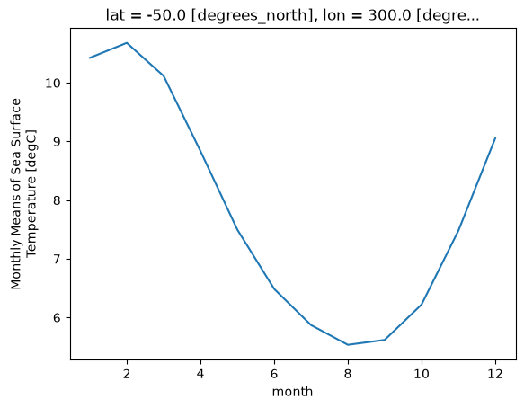
Climatlogy at a specific point in the North Atlantic
sst_mm.sel(lon=300, lat=-50).plot()
plt.show()
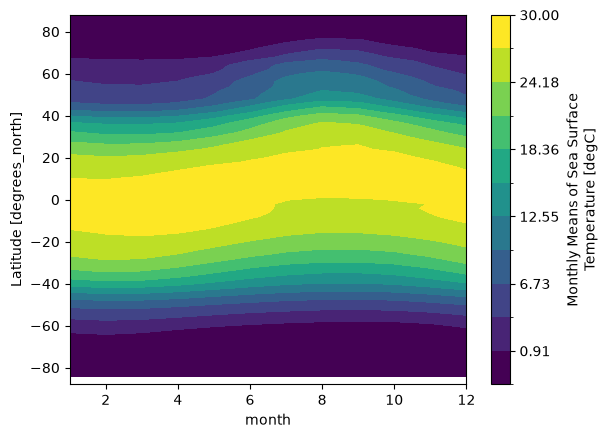
Zonal Mean Climatology
sst_mm.mean(dim='lon').transpose().plot.contourf(levels=12, vmin=-2, vmax=30)
plt.show()
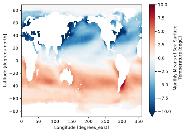
Difference between January and July Climatology
(sst_mm.sel(month=1) - sst_mm.sel(month=7)).plot(vmax=10)
plt.show()
7.3.2.2. Transformations#
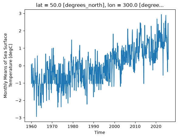
Now we want to remove this climatology from the dataset, to examine the residual, called the anomaly, which is the interesting part from a climate perspective. Removing the seasonal climatology is a perfect example of a transformation: it operates over a group, but doesn’t change the size of the dataset. Here is one way to code it.
def remove_time_mean(x):
    return x - x.mean(dim='time')

ds_anom = noaa_sst.groupby('time.month').map(remove_time_mean)
ds_anom
<xarray.Dataset> Size: 51MB
Dimensions:  (time: 792, lat: 89, lon: 180)
Coordinates:
  * time     (time) datetime64[ns] 6kB 1960-01-01 1960-02-01 ... 2025-12-01
  * lat      (lat) float32 356B 88.0 86.0 84.0 82.0 ... -82.0 -84.0 -86.0 -88.0
  * lon      (lon) float32 720B 0.0 2.0 4.0 6.0 8.0 ... 352.0 354.0 356.0 358.0
Data variables:
    sst      (time, lat, lon) float32 51MB -1.669e-06 0.0 -5.96e-07 ... nan nan
Attributes: (12/39)
    climatology:               Climatology is based on 1971-2000 SST, Xue, Y....
    description:               In situ data: ICOADS2.5 before 2007 and NCEP i...
    keywords_vocabulary:       NASA Global Change Master Directory (GCMD) Sci...
    keywords:                  Earth Science > Oceans > Ocean Temperature > S...
    instrument:                Conventional thermometers
    source_comment:            SSTs were observed by conventional thermometer...
    ...                        ...
    product_version:           Version 6
    history:                   created 01/16/2025 by PSL using NCEI ERSST V6 ...
    References:                https://www.ncdc.noaa.gov/data-access/marineoc...
    summary:                   ERSSTv6 is developped based on v5, by replacin...
    comments:                  SSTs were observed by conventional thermometer...
platform: Ship and Buoy SSTs from ICOADS R3.0.2 and Argo...Note
In the above example, we applied groupby to a Dataset instead of a DataArray.
Xarray makes these sorts of transformations easy by supporting groupby arithmetic. This concept is easiest explained with an example:
gb = noaa_sst.groupby('time.month')
ds_anom = gb - gb.mean(dim='time')
ds_anom
<xarray.Dataset> Size: 51MB
Dimensions:  (lat: 89, lon: 180, time: 792)
Coordinates:
  * lat      (lat) float32 356B 88.0 86.0 84.0 82.0 ... -82.0 -84.0 -86.0 -88.0
  * lon      (lon) float32 720B 0.0 2.0 4.0 6.0 8.0 ... 352.0 354.0 356.0 358.0
  * time     (time) datetime64[ns] 6kB 1960-01-01 1960-02-01 ... 2025-12-01
    month    (time) int64 6kB 1 2 3 4 5 6 7 8 9 10 11 ... 3 4 5 6 7 8 9 10 11 12
Data variables:
    sst      (time, lat, lon) float32 51MB -1.669e-06 0.0 -5.96e-07 ... nan nan
Attributes: (12/39)
    climatology:               Climatology is based on 1971-2000 SST, Xue, Y....
    description:               In situ data: ICOADS2.5 before 2007 and NCEP i...
    keywords_vocabulary:       NASA Global Change Master Directory (GCMD) Sci...
    keywords:                  Earth Science > Oceans > Ocean Temperature > S...
    instrument:                Conventional thermometers
    source_comment:            SSTs were observed by conventional thermometer...
    ...                        ...
    product_version:           Version 6
    history:                   created 01/16/2025 by PSL using NCEI ERSST V6 ...
    References:                https://www.ncdc.noaa.gov/data-access/marineoc...
    summary:                   ERSSTv6 is developped based on v5, by replacin...
    comments:                  SSTs were observed by conventional thermometer...
platform: Ship and Buoy SSTs from ICOADS R3.0.2 and Argo...Now we can view the climate signal without the overwhelming influence of the seasonal cycle.
Timeseries at a single point in the North Atlantic
ds_anom.sst.sel(lon=300, lat=50).plot()
plt.show()
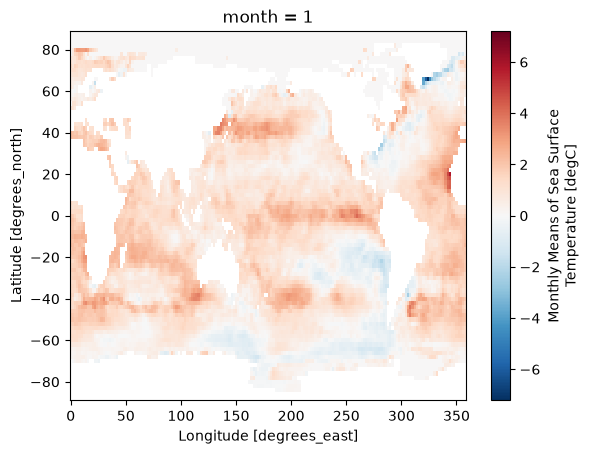
Difference between Jan. 1 2024 and Jan. 1 1960
(ds_anom.sel(time='2024-01-01') - ds_anom.sel(time='1960-01-01')).sst.plot()
plt.show()
7.4. Grouby-Related: Resample, Rolling, Coarsen#
7.4.1. Resample#
Resample in xarray is nearly identical to pandas.
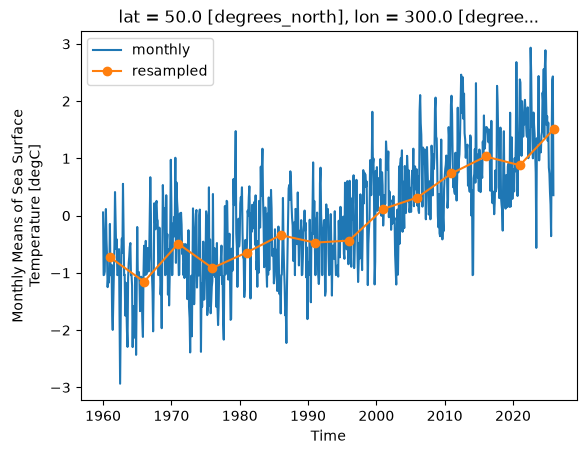
It can be applied only to time-index dimensions. Here we compute the five-year mean.
It is effectively a group-by operation, and uses the same basic syntax.
Note that resampling changes the length of the the output array.
See the list of string aliases for time series frequencies
ds_anom_resample = ds_anom.resample(time='5YE').mean(dim='time')
ds_anom_resample
<xarray.Dataset> Size: 898kB
Dimensions:  (time: 14, lat: 89, lon: 180)
Coordinates:
  * time     (time) datetime64[ns] 112B 1960-12-31 1965-12-31 ... 2025-12-31
  * lat      (lat) float32 356B 88.0 86.0 84.0 82.0 ... -82.0 -84.0 -86.0 -88.0
  * lon      (lon) float32 720B 0.0 2.0 4.0 6.0 8.0 ... 352.0 354.0 356.0 358.0
Data variables:
    sst      (time, lat, lon) float32 897kB -0.003754 -0.003663 ... nan nan
Attributes: (12/39)
    climatology:               Climatology is based on 1971-2000 SST, Xue, Y....
    description:               In situ data: ICOADS2.5 before 2007 and NCEP i...
    keywords_vocabulary:       NASA Global Change Master Directory (GCMD) Sci...
    keywords:                  Earth Science > Oceans > Ocean Temperature > S...
    instrument:                Conventional thermometers
    source_comment:            SSTs were observed by conventional thermometer...
    ...                        ...
    product_version:           Version 6
    history:                   created 01/16/2025 by PSL using NCEI ERSST V6 ...
    References:                https://www.ncdc.noaa.gov/data-access/marineoc...
    summary:                   ERSSTv6 is developped based on v5, by replacin...
    comments:                  SSTs were observed by conventional thermometer...
platform: Ship and Buoy SSTs from ICOADS R3.0.2 and Argo...fig, ax = plt.subplots()
ds_anom.sst.sel(lon=300, lat=50).plot(ax=ax, label='monthly')
ds_anom_resample.sst.sel(lon=300, lat=50).plot(ax=ax, marker='o', label='resampled')
plt.legend()
plt.show()
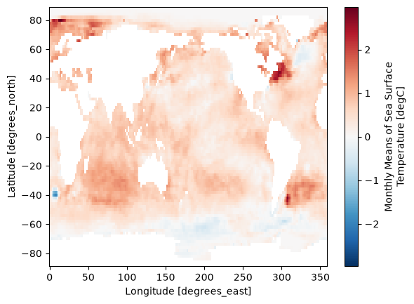
fig, ax = plt.subplots()
(ds_anom_resample.sel(time='2015-01-01', method='nearest') -
 ds_anom_resample.sel(time='1965-01-01', method='nearest')).sst.plot(ax=ax)
plt.show()
7.4.2. Rolling#
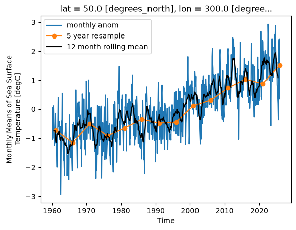
Rolling is also similar to pandas.
It does not change the length of arrays.
Instead, it allows a moving window to be applied to the data at each point.
ds_anom_rolling = ds_anom.rolling(time=12, center=True).mean()
ds_anom_rolling
<xarray.Dataset> Size: 51MB
Dimensions:  (lat: 89, lon: 180, time: 792)
Coordinates:
  * lat      (lat) float32 356B 88.0 86.0 84.0 82.0 ... -82.0 -84.0 -86.0 -88.0
  * lon      (lon) float32 720B 0.0 2.0 4.0 6.0 8.0 ... 352.0 354.0 356.0 358.0
  * time     (time) datetime64[ns] 6kB 1960-01-01 1960-02-01 ... 2025-12-01
    month    (time) int64 6kB 1 2 3 4 5 6 7 8 9 10 11 ... 3 4 5 6 7 8 9 10 11 12
Data variables:
    sst      (time, lat, lon) float32 51MB nan nan nan nan ... nan nan nan nan
Attributes: (12/39)
    climatology:               Climatology is based on 1971-2000 SST, Xue, Y....
    description:               In situ data: ICOADS2.5 before 2007 and NCEP i...
    keywords_vocabulary:       NASA Global Change Master Directory (GCMD) Sci...
    keywords:                  Earth Science > Oceans > Ocean Temperature > S...
    instrument:                Conventional thermometers
    source_comment:            SSTs were observed by conventional thermometer...
    ...                        ...
    product_version:           Version 6
    history:                   created 01/16/2025 by PSL using NCEI ERSST V6 ...
    References:                https://www.ncdc.noaa.gov/data-access/marineoc...
    summary:                   ERSSTv6 is developped based on v5, by replacin...
    comments:                  SSTs were observed by conventional thermometer...
platform: Ship and Buoy SSTs from ICOADS R3.0.2 and Argo...fig, ax = plt.subplots()
ds_anom.sst.sel(lon=300, lat=50).plot(ax=ax, label='monthly anom')
ds_anom_resample.sst.sel(lon=300, lat=50).plot(ax=ax, marker='o', label='5 year resample')
ds_anom_rolling.sst.sel(lon=300, lat=50).plot(ax=ax, label='12 month rolling mean', color='k')
plt.legend()
plt.show()
7.5. Coarsen#
Coarsen is a simple way to reduce the size of your data along one or more axes.
It is very similar to resample when operating on time dimensions; the key difference is that coarsen only operates on fixed blocks of data, irrespective of the coordinate values, while resample actually looks at the coordinates to figure out, e.g. what month a particular data point is in.
For regularly-spaced monthly data beginning in January, the following should be equivalent to annual resampling. However, results would be different for irregularly-spaced data.
noaa_sst.coarsen(time=12, boundary = 'exact').mean()
<xarray.Dataset> Size: 4MB
Dimensions:  (time: 66, lat: 89, lon: 180)
Coordinates:
  * time     (time) datetime64[ns] 528B 1960-06-16T08:00:00 ... 2025-06-16T12...
  * lat      (lat) float32 356B 88.0 86.0 84.0 82.0 ... -82.0 -84.0 -86.0 -88.0
  * lon      (lon) float32 720B 0.0 2.0 4.0 6.0 8.0 ... 352.0 354.0 356.0 358.0
Data variables:
    sst      (time, lat, lon) float32 4MB -1.76 -1.737 -1.732 ... nan nan nan
Attributes: (12/39)
    climatology:               Climatology is based on 1971-2000 SST, Xue, Y....
    description:               In situ data: ICOADS2.5 before 2007 and NCEP i...
    keywords_vocabulary:       NASA Global Change Master Directory (GCMD) Sci...
    keywords:                  Earth Science > Oceans > Ocean Temperature > S...
    instrument:                Conventional thermometers
    source_comment:            SSTs were observed by conventional thermometer...
    ...                        ...
    product_version:           Version 6
    history:                   created 01/16/2025 by PSL using NCEI ERSST V6 ...
    References:                https://www.ncdc.noaa.gov/data-access/marineoc...
    summary:                   ERSSTv6 is developped based on v5, by replacin...
    comments:                  SSTs were observed by conventional thermometer...
platform: Ship and Buoy SSTs from ICOADS R3.0.2 and Argo...Coarsen also works on spatial coordinates (or any coordiantes).
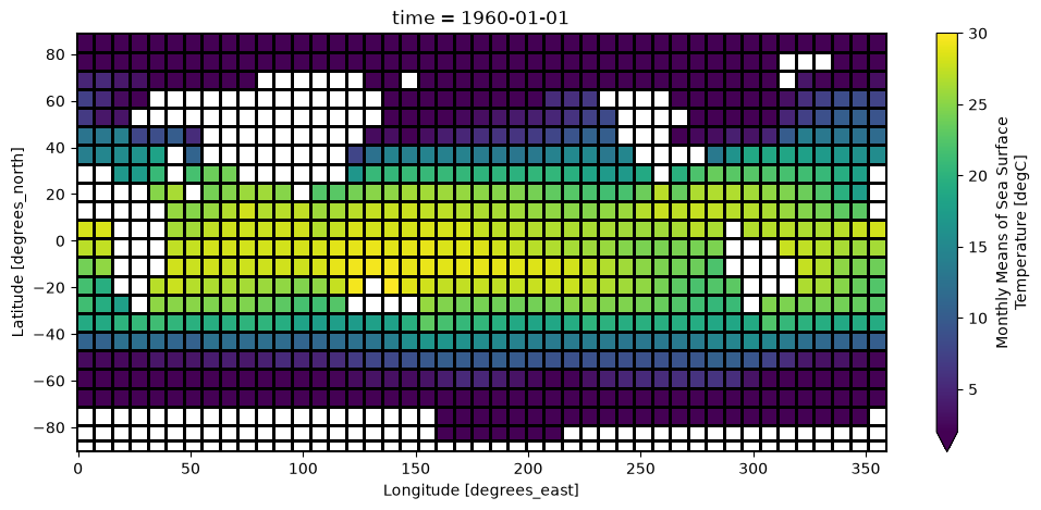
fig, ax = plt.subplots(figsize=(12, 5))
ds_coarse = noaa_sst.coarsen(lon=4, lat=4, boundary='pad').mean()
ds_coarse.sst.isel(time=0).plot(ax=ax, vmin=2, vmax=30, edgecolor='k')
plt.show()